To help the user visualize the study and results, LifeSim has the capability to display map layers that represent the features of a study. The map
layers displayed in the map window are also listed in the Map Layers tab. Map layers provide
a geographical reference for the study area. The LifeSim GUI (Figure) describes the formats of the map layers, and
provides commands that allow the user to configure, manage, and edit map layers.
Figure: LifeSim Main Window
Map layers are optional and not necessary for computing and reviewing results (see Viewing LifeSim
Results). However, to view the results of simulation animations (View Result Map In the Map
Window), the map window is useful for helping to facilitate the review of simulation results and discussion with
emergency managers. Furthermore, viewing map layers in the map window is a useful way to examine the validity of imported datasets. For example, a
road network with missing connectivity or incorrect directions on one-way roads can lead to erroneous results. Therefore, editing the road network
dataset can provide a reliable foundation for traffic simulation (Appendix
C provides an example of editing an imported
road network dataset in the map window).
The map window (Figure) provides a way to graphically display LifeSim components. The rendering engine takes advantage
of the computers graphics processing using Open Graphics Library - OpenGL to draw the map layers. All geographic information system (GIS) data is
re-projected on the fly using GDAL (Geospatial Data Abstraction Library).
There are two toolbars located in the Map Toolbar (Figure): the General
Toolbar and the Editor Toolbar (Figure). Details about each toolbar are detailed in the following sections.
Figure: LifeSim Map Toolbar: General Toolbar and Editor Toolbar
The General Toolbar includes the Select Tool (B), Pan Tool (P), Zoom In Tool (Z), Zoom to full extents, Add Data, Query Features Tool (Q), and Measure
Distance Tool (M). These tools change the appearance of the cursor, as well as the functionality of the mouse cursor in the map window.
Table: LifeSim General Toolbar - Available Tools and Functionality
Tool
Functionality
Select Tool (B)
Select elements displayed in the Map Window. To select features, click on a feature or click, hold, and drag a rectangle around features to select them in the Map Window. Additionally, the Select tool allows users to access shortcut menus which can be customized when in editing mode. Refer to Appendix B for more information regarding editing mode.
Pan Tool (P)
Pan the Map Window; click the Pan tool and click, hold and move the mouse around the Map Window. Also, if the mouse has a wheel, then the user can pan the Map Window by using the wheel (click and hold the wheel to pan).
Zoom In Tool (Z)
Zoom in to areas of the Map Window. To zoom in, hold the mouse button down and outline the area of interest to enlarge. Also, if the mouse has a wheel, then the user can zoom in or out using the wheel (wheel up zooms in and wheel down zooms out).
Fixed Zoom Out Tool (O)
Zooms out to a fixed distance. Click the Fixed Zoom Out tool once and the Map Window view will zoom out a fixed distance. Double-click on the tool icon, and the Map Window view will zoom out twice the fixed distance. Additionally, the user can utilize the shortcut menu option: right-click anywhere in the Map Window to zoom in or out a fixed distance.
Zoom to full extents
A quick way to re-center the map by zooming out to the full geo-graphical extent of the map layers in the Map Window. Web layers do not affect the map extents.
Add Data
After clicking the Add Data tool, the File Explorer browser window will open. This browser allows users to navigate to layers (including *.shp, *.flt, *.tif, and *.vrt) of interest and add the layer(s) to the map window.
If the user clicks the down arrow next to the Add Data tool, a shortcut menu will appear which allows the user to Add New [Data], Add Web Imagery, or Create New [Vector Features File] that is added to the Map Window.
Query Features Tool (Q)
Identifies the geographic feature or place currently selected in the Map Window. Alternatively, multiple features can be identified by dragging a box over the desired area. Once a selection is made, the Feature Query dialog box will open with the information presented in table format separated by Feature type. Only visible layers in the Map Window will be queried.
Measure Distance Tool (M)
Measure the distance along a specified line. With the tool selected, click to initiate the measure line. Each subsequent click will add a new point to the measure line. When finished, double-click on the location of the final point. The Measure Results dialog box will open and display the distance in the units the user has chosen (feet, miles, meters, or kilometers).
The set of tools located in the Editor Toolbar become active after users initiate an editing session for a map layer. When a user
right-clicks on a map layer in the Map Layers tab, from the shortcut menu (Figure),
click Edit, and the tools in the Editor Toolbar become active. Only one map layer can be edited at one time. For
lines and polygons, there are two editing modes: feature edit and vertex edit. Clicking on a selected feature puts the user into the feature edit
mode (move, delete, reverse), and double-clicking on a selected feature puts the user in the vertex edit mode (add, delete, edit vertex points).
There are some tools available during an edit session which are not available from the shortcut menu or the
Editor Toolbar. Clicking Delete will delete all currently selected features or currently selected vertices depending
on which mode the user is in. Clicking the R key will reverse the direction of a currently selected line feature. Also,
right-clicking during an edit session allows the user to do multiple tasks depending on what is clicked.
Figure: Individual Map Layer Shortcut Menu
Table: LifeSim Editor Toolbar - Available Tools and Functionality
Tool
Functionality
Add new features (A)
Add a new feature to the editable map layer by left-clicking to add feature data. Selected features can be deleted by either clicking the Delete key, or right-click on the selected feature(s) and from the shortcut menu, click Delete Selected Features.
Insert vertex (I)
Add a vertex to an existing line or polygon map layer. The tool becomes available when the selected feature is in vertex edit mode. As the cursor gets close to the line or polygon edge, the Map Window will display what the updated feature will look like if a vertex is added at the cursor. Left-click to insert the new vertex.
Break line feature into two... (K)
Split a line feature into two features at the point the user clicked on the line. The user needs to be in the feature edit mode for this tool to be enabled.
Continue from end (lines only)
Continue a line feature from the end point of the line feature to the point to a second point clicked in the Map Window. Double-click to finish the line continuation edits or right-click and choose Finish Editing Vertices or choose a different tool to finish the line continuation. The user needs to be in the vertex edit mode for this tool to be enabled.
Add new line or polygon to existing feature
Add a polygon or line to an existing selected polygon or line feature. For example, to add a hole to a polygon, click to add points defining the hole and double-click to finish. The user needs to be in the vertex edit mode for this tool to be enabled.
Feature Snapping Settings
Define snapping rules when editing. Snapping will automatically move the desired action to the nearest snap point when the cursor is close. This can be very useful when trying to line up endpoints of line features or place points directly on top of other features. Enable snapping by clicking Enable Snapping. From the Snap to Layer list, select the desired feature to snap to, then select under Snapping Options how snapping will be applied (to all points, end points, or edges).
Undo (Ctrl + Z)
Undo changes made during an edit session. Only enabled if there are edits that can be undone.
Redo (Ctrl + Y)
Redo changes made. Only enabled if there are edits to redo.
Save Edits (Ctrl + S)
Saves all edits made during the editing session. Only enabled if edits have been made.
Stop Editing
Stops the edit session. At this point a new map layer can be selected for editing. If edits have been made, then the user will be prompted to save them before stopping the edit session.
If a tool has a parentheses after the tooltip, the letter in the parentheses represents a hot key (Table) to call on
the tool without clicking on it. For example, for the Query Features tool, if the user clicks Shift-Q over the map window, the
Query Features tool will be active.
NOTE: for the hot keys to work for tools located in the Editor Toolbar, users must first
initiate an editing session for a map layer.
To set the projection (coordinate system) associated with the LifeSim study, from the LifeSim main window, from
the Mapping menu (Figure), click Map Properties. The Map Properties
dialog box will open (Figure). From this dialog box, the user can setup the projection for the LifeSim study.
Figure: Mapping Menu
1From the Map Properties dialog box, click Set Fixed Projection (Figure).
Figure: Mapping Properties Dialog Box
2An Open browser will open (Figure). From the Open browser, navigate to the projection file of interest (usually any shapefile associated with the study area), select a projection file (*.prj), and click Open.
Figure: Open Browser
3The Open browser will close, and the projection for the study will now be displayed in the Map Properties dialog box (Figure). Click OK, and the Map Properties dialog box will close.
Figure: Map Properties Dialog Box - Projection Example
The Map Layers tab (Figure) provides a tree view for the map layers that have been added to an
LifeSim study. However, only selected () layers
in the Map Layers tab will display in the map window (Figure). The user can turn map layers
on or off, adjust the properties of the layers, and modify the order of the layers for viewing in the map window.
Geographic Information System (GIS) files are the map layer formats supported by LifeSim and include: *.shp, *.flt, *.tif,
and *.vrt. The user can add map layers, add background map layers, remove map layers, adjust a map layer's position in the view, edit a map
layer's properties, zoom into a layer, and many other functions. The ability to manipulate the different map layers is specific for that map layer
format.
1From the LifeSim main window, from the Mapping menu (Figure), click Add Map Layer. Another way is from the General Toolbar (Figure), click . Either way, the Browse for files browser (Figure) will open.
Figure: Browse for files Browser Window
2From the Browse for files browser (Figure), navigate to the GIS file of interest that will be added as a map layer. Select the appropriate GIS file (*.shp, *.flt, *.tif, or *.vrt) and the File name box will now display the selected file name.
3Click Open, and the Browse for files browser (Figure) will close. The selected dataset will now be displayed in the map window, and the selected map layer name will appear in the Map Layer Tree.
Knowing where the study is located in reference to known geographic positions can be quite helpful with communication. There are two types of internet
background maps: OpenStreetMap and ESRI World Imagery map. There are two ways to add these background internet
maps.
To add a background internet map to the LifeSim study, from the Mapping menu (Figure), point to Add Web
Layer, and select the internet map from the available list that would be a good
background map for the study area. Another way is from the General Toolbar,
click the Add Data dropdown menu, point
to Add Web Imagery (Figure), and
select the internet map from the available list that would be a good background map for the study area. Either way, the selected background map
displays in the map window (e.g., ESRI World Imagery in Figure).
Figure: Mapping Menu - General Toolbar - Add Web Imagery Options
Once a map layer is added to a LifeSim study, the user can adjust the position of a map layer. Within the LifeSim framework, some map layers represent
a particular LifeSim dataset (i.e., hydraulic data, structure inventories, emergency planning zones), while other map layers provide information.
The Map Layer Tree (Figure) displays the map layers from top to bottom, where the top-most layer
overlays the next one down in the list and continues to the bottom layer. If a background internet map is added from the Add
Data dropdown menu , that map layer
will automatically be added to the bottom of the Map Layer Tree and will be underneath all layers listed above the internet map. At times, it may be
desirable to have various
map layers drawn in a different order in the map window.
To move map layers:
1From the Map Layer Tree (Figure), right-click on the map layer of interest. From the shortcut menu (Figure), either select Move Up or Move Down.
Figure: LifeSim Main Window - Map Layers Tree - Internet Map Shortcut Menu
2To move the map layer of interest below other map layers listed in the Map Layer Tree, click Move Down. The selected map layer will move one step below its current position. Repeat until the map layer of interest is at the desired location within the Map Layer Tree.
3To move the map layer of interest above other map layers listed in the Map Layer Tree, click Move Up. The selected map layer will move one step above its current position. Repeat until the map layer of interest is at the desired location within the Map Layer Tree.
Another way to move map layers in the Map Layer Tree is to drag and drop a map layer to the desired location within
the Map Layer Tree. Click and hold the map layer of interest, and move the cursor up or down the Map Layer
Tree (the selected map layer will move in conjunction with the mouse). A bar will show the new location where the selected map layer
will be moved (Figure). Release the mouse, and the selected map layer will be in a new position.
Figure: Drag and Drop: Moving a Selected Map Layer in the Map Layers Tree
This option will set the zoom of the map window based on the extents of the selected map layer. From the Map Layer
Tree, right-click on the map layer of interest (Figure). From the shortcut menu, click Zoom to
Layer. The map window view will change to include the entire extent for
the selected map layer.
There are three options (SelectAll, Select byPolygon, or Reverse
Selection) for selecting map layer features from the individual map layer shortcut menu (Figure).
Table describes the Select sub-menu commands.
Figure: Individual Map Layer Shortcut Menu - Select Options
Table: Select Sub-Menu Commands
Command
Description
Select All
The Select All command will select all of the features within the map layer.
Select by Polygon
The Select by Polygon command will open the Select by Polygon dialog box (Figure).
Reverse Selection
The Reverse Selection command will select the opposite. For example, if all of the features are selected in the map layer, then choosing Reverse Selection will de-select all of the features.
1From the Map Layers tab, right-click on a map layer of interest (Figure). From the shortcut menu, point to Select, and click Select by Polygon. The Select by Polygon dialog box will open (Figure).
Figure: Select by Polygon Dialog Box
2From the Selection Polygon box (Figure), the user must select either Polygon from map or Polygon from file.
aPolygon from map (default): The user will need to select a polygon map layer that is part of the LifeSim study from the Polygon map layer list (Figure), which contains a list of the polygon map layers (e.g., the Emergency Planning Zone(s) map layer) presently in the Map Layers tab. Notice, there is an option in the Polygon from map section to Use selected polygons (Figure). The Use selected polygons option will only be available when the identified Polygon map layer has features selected or if a subset of a layer has been selected (using the Select By Attribute option is explained in Map Layer Attributes Dialog Box; or the map layer Select options are explained in Map Layer Select Options).
bPolygon from file: This allows the user to select a polygon shapefile. When selected, from the Polygon shapefile box (Figure), click . The Select a Polygon Shapefile browser will open. The user will need to navigate to the file of choice and select the desired polygon shapefile (*.shp). Click Open, the Select a Polygon Shapefile browser will close, and the name of the selected polygon shapefile will display in the Polygon shapefile box (Figure).
Figure: Select by Polygon Dialog Box - Polygon from file option
3Next, from the Selection Options box (Figure), the user needs to set the selection type. The choices are Contains and Intersects.
aContains (default): this option will select features that are completely within a polygon that has been selected. In other words, this option will not select any features which intersected with the border of the selecting polygon.
bIntersects: this option will only select features which intersects the polygon that has been selected. This includes features that are completely contained in the selection polygon in addition to intersecting with the border of the selecting polygon. NOTE: this option will is not available for point shapefiles.
4The last step is the Selections Method (Figure). Available options are Append, New Selection, and Select from Selection.
aAppend: this option adds the selection to the already selected features. This option will only be available if there are selected features within the input map layer.
bNew Selection (default): this option will clear any previous selection made to the input map layer.
cSelect from Selection: this option will only select features that are currently selected in the input map layer.
5Click OK (Figure), and the Select by Polygon dialog box will close. Now, the selected map layer will have features selected in the map window corresponding to the preferences set in the Select by Polygon dialog box.
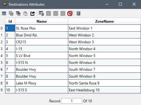
Map layer attributes can be accessed for each map layer and provides a table for the dataset referenced by the map layer.
To access a specific map layer Attributes table: from the Map Layers tab, right-click on a map layer of interest. From the
shortcut menu (Figure), click Open Attribute
Table. The Map Layer Attributes dialog box will open (Figure). Editing of the map layer attributes is detailed in
Editing Map Layer Features and Attributes of this appendix.
Figure: Map Layer Attributes Dialog Box
NOTE: from the table, when a single cell is selected (e.g., row 1, column 1 in Figure), the keyboard arrow keys (and the tab and enter keys)
can be utilized to step through the table one cell at a time.
Table describes the functionality of the Export and Copy Tools toolbar.
Table: LifeSim Export and Copy Tools - Available Tools and Functionality
Tool
Functionality
Select all cells
Selects all cells in the table.
Copy Selected Cells
Copies cells selected in the table. The information is copied to the clipboard and needs to be pasted to another application (e.g., Microsoft Excel®) for saving.
Copy Selected Cells with Table Headers
Copies cells selected in the table and the table headers. The information is copied to the clipboard and needs to be pasted to another application (e.g., Microsoft Excel®) for saving.
Paste from the Clipboard into the Table
Pastes data copied from another table into the current table.
Export Table
Opens a Save As browser window, which allows the user to export the data in the table to a Microsoft Excel® (*.xlsx) file.
Table describes the functionality of the Selection Tools toolbar.
Table: LifeSim Table Selection Tools - Available Tools and Functionality
Tool
Functionality
Select Rows By Attribute
Opens the Select By Attribute dialog box (Figure), which allows the user to perform queries, make selections, and locate features in the table. When a feature is selected in the attribute table, that same feature will also be selected in the map window (and vice versa).
Show All Rows
Display all rows (selected or unselected) in the table.
Show Selected Rows Only
Only display features selected in the table.
Deselect All Rows
Unselects all rows which were selected in the table.
To access and select specific attributes for a map layer:
1From the Map Layers tab of the LifeSim main window (Figure), right-click on the map layer of interest. From the shortcut menu (Figure), click Open Attribute Table. The Map Layer Attributes dialog box will open (Figure)
2Click . The Select By Attribute dialog box opens (Figure). By selecting certain attributes and using expressions, the user can manipulate the selected map layer. The Available Columns box (Figure) provides a list of all of the attributes fields of the selected map layer. Double-click on an attribute in the Available Columns box. This will add the attribute to the Expression box (Figure).
3The Functions button (Figure) opens a new window providing a selection of all available functions in LifeSim. Select a function from the Functions list (e.g., AND in Figure) to view tips for using the function. Click Insert to add the selected function to the Expression box (Figure).
Figure: Select by Attribute - Functions
4Figure provides an example expression for selecting attributes in the table that satisfy the entered expression. The expression was entered by selecting AND from the Functions list (Figure); Stories_Number and DayU65Population from the Available Columns (Figure) list; and has set Stories_Number equal to 1 and DayU65Population greater than 100.
Figure: Select By Attribute Dialog Box - Example ExpressionA message appears below the Expression box (Figure): Example: First data record (row id = 0) would NOT get selected.
In other words, the first row within the attribute table does not satisfy the expression; therefore, the first row in the attributes table will not become selected when the Execute (Figure) button is clicked. On the other hand, if the first row did satisfy the expression, then the message would say Example: First data record (row id = 0) WOULD get selected, and the first row in the attribute table would become selected when the Execute (Figure) button is clicked.
5If the entered expression contains errors, the message section will display the issues with the expression. The message will say Errors found in expression until the expression is completed correctly (Figure).
Figure: Select By Attribute Dialog Box - Error Message
6Another resource providing help to complete an expression is the Error Log button, which is available when an expression is incorrect. Click Error Log, and the Errors Encountered in Expression dialog box will open (Figure). Information is provided on what the possible issues are with the defined expression.
Figure: Errors Encountered in Expression in Dialog Box
7Once the expression is correct, click Execute to run the expression (Figure). The Select By Attribute dialog box (Figure) will close, and the rows in the table of the Map Layer Attributes dialog box where the expression is True will be highlighted in dark teal (Figure). Additionally, the Show Selected Rows Only and Deselect All Rows icons are now active.
8After a selection is made in the table, the feature is not only highlighted in the table (Figure), but is also highlighted in the map window for the selected map layer. For example, in Figure, features are highlighted in the map window following the successful execution of the defined expression. The highlighted features will be differentiated in bright teal (as opposed to the original blue color). Double-clicking in the map window will deselect the features.
Figure: Map Window - Displaying Selected Features
9Show Selected Rows Only will only display the highlighted features in the table of the Map Layer Attributes dialog box (Figure). Clicking
(Show All Rows) will bring back all of the records for the selected map layer.
Other functions and commands are available from the Map Layer Attributes dialog box (Figure).
If the user right-clicks on a selected row in the table, a shortcut menu will display with one option: Zoom to
Selected (left popup within Figure). Zoom to Selected will zoom the map window view to the
features selected in the table.
When the user right-clicks on selected column(s) in the table, a shortcut menu will display with several
available options: Sort Ascending, Sort Descending, Remove Sort, Summary Statistics, Find, Field Calculator,
and Delete Column (center popup within Figure). Other options are
available when the user is in edit mode (described in Editing in the Attribute
Table).
Sort Ascending
Sort Descending
Remove Sort
Summary Statistics
Find
Sorts the selected column in ascending (i.e., low to high; A to F) order. After clicking Sort Ascending, an up arrow displays in the column header (e.g., Stories_Number in Figure) to show the sorting of the selected column. Double-clicking on a selected column will reverse the current sort.
Sorts the selected column in descending (i.e., high to low; F to A) order. After clicking Sort Descending, a down arrow displays in the column header to show the sorting of the selected column. Double-clicking on a selected column will reverse the current sort.
Remove Sort does not become active until either Sort Ascending or Sort Descending has been clicked. Remove Sort will revert the selected column back to its original state.
When clicked, the Attribute Summary Statistics dialog box will open (Figure), providing the summary statistics for the selected column in the table. If the selected column has numeric values, then the summary statistics will include indicative statistics of the data and a histogram (similar to Figure). If the selected columns have text data, then the summary statistics will have a list of all the unique text values and the frequency of those text values along with a pie chart of the most frequent text values. When rows in the table on the Map Layer Attributes dialog box (Figure) are selected, the Selected Rows Only option (Figure) becomes available in the Attribute Summary Statistics dialog box (Figure). If the user clicks this option, the summary statistics displayed are only for the selected rows in the Map Layer Attributes table (Figure). The pie chart will lump smaller counts into a new unique value and count entitled Other if there are more than four unique items associated with the selected column.Figure: Attributes Summary Statistics Dialog Box
The Find option is only available when the entire table on the Map Layer Attributes dialog box (Figure) is available. If the user has selected Show Selected Rows Only (Figure), then the Find option will not be available. When Find is clicked, the Find In: Attribute dialog box (Figure) will open. The user can search for specific attributes by entering the attribute name in the Find box.Figure: Find In: Attribute Dialog Box
New map layers can be created in LifeSim using the Create New Vector Features File dialog box (Figure). The new
map layers created are shapefiles (*.shp) which store non-topological geometry and attribute information for the spatial features
of a dataset.
Figure: Create New Vector Features File Dialog Box
To create a new map layer:
1From the LifeSim main window, from the Mapping menu (Figure), click Create New Vector Layer. Another way is from the General Toolbar, click the Add Data tool; from the shortcut menu, click Create New (Figure). Either way, the Create New Vector Features File dialog box (Figure) will open.
Figure: Mapping MenuFigure: General Toolbar – Add Data Shortcut Menu
2From the File Output Location box (Figure), click . A Save As browser will open (Figure). Navigate to the desired directory for storing the shapefile (*.shp). Enter a name (required) in the File name box (Figure) for the new map layer. Click Save. The Save As browser will close, and the path name and file name of the new map layer will display in the File Output Location box (Figure).
Figure: Save as Browser
3From the Feature Type dropdown list (Figure), select the geographic features of the shapefile which can be represented as points, polylines (lines), or polygons (areas).
aPoint: Features that are too small to be represented by lines or polygons. Examples include structure inventories and destinations.
bPolyline: Features that represent the shape and location of geographic objects, such as the road networks.
cPolygon: A set of many-sided area features which represent the shape and location of a feature or set of features, such as emergency planning zone(s).
4Users have the option to select a projection for the new map layer from another map layer. To add a reference map coordinate system (create a projection), from the Projection box (Figure), click . An Open browser will open (Figure). Navigate to the location of the projection file that contains the projection that will be used for the new map layer (*.prj), select the file, and click Open. The Open browser will close, and the Create New Vector Features File dialog box Projection will now contain the file location of the selected projection file (Figure).
5Click OK, and the Create New Vector Features File dialog box (Figure) will close. The LifeSim Map Layers tab (Figure) will now contain the newly created map layer.
6The next step after creating a new map layer is to add new features. Adding new features to the map layer will be discussed in detail in Editing Map Layer Features and Attributes.
1From the LifeSim main window, from the Mapping menu, point to Remove Map Layer (Figure). From the list of map layers, click on the map layer that is to be removed from the LifeSim study. The map layer is removed.
Figure: Mapping Menu - Remove Map Layer
2Another option is from the LifeSim main window, from the Map Layers tab, right-click on the map layer of interest (Figure). From the shortcut menu, click Remove. The selected map layer will be removed from the LifeSim study. Remove will allow the user to select multiple map layers for removal.
In LifeSim, there are tools available to perform operations on map layers that can be useful in preparing data and analyzing results (e.g., exporting
shapefiles, clipping features, or creating buffer polygons). Currently, tools are only available for points, lines, and polygons shapefiles but will be
expanded in the future to include gridded data.
From the Map Layers tab on the LifeSim main window (Figure)
right-click on a map layer of interest. From the shortcut
menu, point on Tools, from the
submenu (Figure) are several commands that are available for editing map layers. These commands change according to the
feature type (points, polylines, or polygons).
Figure: Individual Map Layer Shortcut Menu - Tools Sub-menu Commands
The following is an overview of each command:
Export to New Shape
Buffer
Create Centroids Shapefile
Clip
Simplify
Exports the selected map layer as a new shapefile (i.e., output shapefile), saved with a name provided by the user. There are options to save the new shapefile with the map window projected coordinate system or the original coordinate system set for the selected map layer. Another alternative is to export only selected features for the map layer when a subset of the map layer's features has been selected. This command is available for points, polylines, and polygon feature types. See Export to New Shapefile for further details on the use of this command.
Creates polygons around features within the selected map layer for a set distance around the object called a buffer (Figure). There is an option to merge the buffered features in the created polygon shapefile. If the merge option is selected, all overlapping buffer polygons will be merged into one features and all attribute information will be removed from all of the new buffered features of the created polygon shapefile. This command is available for points, polylines, and polygon feature types. See Buffer for further details on the use of this command.Figure: Buffer Tool Options - Illustration by Feature Type
Calculates the center point for the polygon(s) in the selected map layer and creates a centroids shapefile. An additional option allows the user to only include selected features in the centroid’s shapefile. This command is only available for polygon feature types. See Create Centroids Shapefile for further details on the use of this command.
Clip can be utilized to extract features from the selected map layer using a polygon map layer or polygon shapefile to clip the input map layer features to within the polygon boundaries (Figure). This command is available for polylines and polygon feature types. See Clip Tool for further details on the use of this command.Figure: Clip Tool – Illustration by Feature Type
Simplify is utilized for simplifying the source polyline or polygon map feature by eliminating points based on the Simplification Method chosen. There are three methods to choose from: Visalingam Whyatt, Lang, and Douglas Peucker. Based on the Simplification Method chosen, the dialog box will change to accommodate the parameters for the method of choice. This command is available for polylines and polygon feature types. See Simplify for further details on the use of this command.
To export a selected map layer to a new shapefile:
1From the Map Layers tab, right-click on the map layer of interest (Figure). From the shortcut menu, click Export to New Shape. The Export To Shapefile dialog box will open (Figure).
Figure: Export to Shapefile Dialog Box
2From the Output Shapefile box (Figure), click . A Save As browser will open (Figure). Navigate to the desired location for storing the new shapefile (*.shp), and enter a name (required) in the File name box for the new shapefile.
3Click Save. The Save As browser (Figure) will close, and the Export To Shapefile dialog box (Figure) will now display the path and name for the new shapefile to be saved in the Output Shapefile box.
4Next, the user needs to select the projection for the new shapefile. From the Output Projection box (Figure), the available options are Use Map Projection or Use Source Projection.
aUse Map Projection: this will set the new shapefile's projected coordinate system to that of the LifeSim study.
bUse Source Projection: this will set the new shapefile's projected coordinate system to that of the selected map layer.
5An optional step -- Export Selected Features (Figure) -- allows the user to save the new shapefile with only features that have been selected for the selected map layer (i.e., using the Select By Attribute option explained in Map Layer Attributes Dialog Box; or the Select options explained in Map Layer Select Options).
6Click OK, and the Verify Add Results message window (Figure) will open asking the user if the newly created shapefile should be added to the map window. Click Yes to add the new shapefile to the map window, and the Verify Add Results message window will close.
To create a centroids shapefile from a selected map layer (polygon shapefile):
1From the Map Layers tab, right-click on the map layer of interest (Figure). From the shortcut menu, click Create Centroids Shapefile. The Create Centroids dialog box will open (Figure).
Figure: Create Centroids Dialog Box
2From the Output Shapefile box (Figure), click . A Save As browser will open (Figure). Navigate to the desired location for storing the new centroids shapefile (*.shp), and enter a name (required) in the File name box for the new centroids shapefile.
3Click Save, and the Save As browser (Figure) will close. The Create Centroids dialog box (Figure) will now display the path and shapefile name for the new centroids shapefile to be saved in the Output Shapefile box.
4Next, the user needs to select the projection for the new centroids shapefile. From the Output Projection box (Figure), the available options are Use Map Projection or Use Source Projection.
aUse Map Projection: this will set the new shapefile's projected coordinate system to that of the LifeSim study.
bUse Source Projection: this will set the new shapefile's projected coordinate system to that of the selected map layer.
5An optional step -- Only for Selected Features (Figure) -- allows the user to save the new shapefile with only features that have been selected for the selected map layer (i.e., using the Select By Attribute option explained in Map Layer Attributes Dialog Box; or the Select options explained in Map Layer Select Options).
6Click OK. The Verify Add Results message window (Figure) will open asking the user if the newly created shapefile should be added to the map window. Click Yes to add the new shapefile to the map window. The Verify Add Results message window will close, and the new centroid shapefile will display.
To create a new shapefile that is based one set distance of a selected map layer:
1From the Map Layers tab, right-click on the map layer of interest (Figure). From the shortcut menu, click Buffer. The Create Buffers Polygon(s) dialog box will open (Figure).
Figure: Create Buffer Polygon(s) Dialog Box
2From the Output Shapefile box (Figure), click . A Save As browser will open (Figure). Navigate to the desired location for storing the new shapefile (*.shp), and enter a name (required) in the File name box for the new shapefile.
3Click Save, and the Save As browser (Figure) will close. The Create Buffer Polygon(s) dialog box (Figure) will now display the path and shapefile name for the new shapefile to be saved in the Output Shapefile box.
4Next, the user needs to select the projection for the new shapefile. From the Output Projection box (Figure), the available options are Use Map Projection or Use Source Projection.
aUse Map Projection: this will set the new shapefile's projected coordinate system to that of the LifeSim study.
bUse Source Projection: this will set the new shapefile's projected coordinate system to that of the selected map layer.
5The user will need to enter the buffer distance for the new shapefile. Under Buffer Options (Figure), in the Buffer Distance box, enter the buffer distance in feet (e.g., 50).
6An optional step -- Only Buffer Selected Features (Figure) -- allows the user to save the new shapefile with only features that have been selected for the selected map layer (i.e., using the Select By Attribute option explained in Map Layer Attributes Dialog Box; or the Select options explained in Map Layer Select Options).
7Click OK. The Verify Add Results message window (Figure) will open asking the user if the newly created shapefile should be added to the map window. Click Yes to add the new shapefile to the map window. The Verify Add Results message window will close, and the new shapefile will display.
To create a shapefile of a selected map layer that has been clipped (points and polygons):
1From the Map Layers tab, right-click on the map layer of interest (Figure). From the shortcut menu, click Clip. The Clip by Polygon dialog box will open (Figure).
Figure: Clip by Polygon Dialog Box
2From the Output Shapefile box (Figure), click . A Save As browser will open (Figure). Navigate to the desired location for storing the new shapefile (*.shp), and enter a name (required) in the File name box for the new shapefile.
3Click Save, and the Save As browser (Figure) will close. The Clip by Polygon dialog box (Figure) will now display the path and shapefile name for the new shapefile to be saved in the Output Shapefile box.
4Next, the user needs to clip the selected map layer based on polygon shapefiles that are part of the LifeSim study or from other polygon shapefiles. The available options are: Polygon From Map or Polygon From File.
aPolygon From Map: under the Clip Polygon box (Figure), from the Clip Polygon Shapefile list, all polygon map layers (e.g., an Emergency Planning Zone) imported in the current LifeSim study will be available. Select the desired polygon map layer to clip the selected map layer. An optional feature is Use Selected polygons for clip (Figure), which is only available when the selected map layer has features selected (i.e., using the Select By Attribute option explained in Map Layer Attributes Dialog Box; or the Select options explained in Map Layer Select Options).
bPolygon From File: under the Clip Polygon box (Figure), select Polygon From File. From the Clip Polygon Shapefile box, click . The Please select a clip polygon shapefile browser will open. Navigate to the file of choice and select the desired polygon shapefile (*.shp). Click Open. If the selected file is a polygon shapefile, the Please select a clip polygon shapefile browser will close, and the selected file's path and name will display in the Clip Polygon Shapefile box (Figure). However, if the file selected is not a polygon shapefile, then a warning message window will open (Figure).
Figure: Clip by Polygon Dialog Box - Polygon from File OptionFigure: OpenGLMapping Warning Message
5Next, the user needs to select the projection for the new shapefile. From the Output Projection box (Figure), the available options are Use Map Projection or Use Source Projection.
aUse Map Projection: this will set the new shapefile's projected coordinate system to that of the LifeSim study.
bUse Source Projection: this will set the new shapefile's projected coordinate system to that of the selected map layer.
6An optional step -- Only Clip Selected Features (Figure) -- allows the user to save the new shapefile with only features that have been selected for the selected map layer (i.e., using the Select By Attribute option explained in Map Layer Attributes Dialog Box; or the Select options explained in Map Layer Select Options).
7Click OK. The Verify Add Results message window (Figure) will open asking the user if the newly created shapefile should be added to the map window. Click Yes to add the new shapefile to the map window. The Verify Add Results message window will close, and the new shapefile will display.
To create a shapefile of a selected polygon map layer that has been simplified (polylines and polygons):
1From the Map Layers tab, right-click on the map layer of interest (Figure). From the shortcut menu, click Simplify. The Simplify Polygon(s) dialog box (Figure) will open.
Figure: Simplify Polygon(s) Dialog Box
2From the Output Shapefile box (Figure), click . A Save As browser will open (Figure). Navigate to the desired location for storing the new shapefile (*.shp), and enter a name (required) in the File name box for the new shapefile.
3Click Save, and the Save As browser (Figure) will close. The Simplify Polygon(s) dialog box (Figure) will now display the path and shapefile name for the new shapefile to be saved in the Output Shapefile box.
4Next, the user needs to select the projection for the new shapefile. From the Output Projection box (Figure), the available options are Use Map Projection or Use Source Projection.
aUse Map Projection: this will set the new shapefile's projected coordinate system to that of the LifeSim study.
bUse Source Projection: this will set the new shapefile's projected coordinate system to that of the selected map layer.
5The user must select method for simplifying the selected map layer. Under the Simplify Options box (Figure), from the Simplification Method list, select the appropriate simplification method. Each method has its own set of inputs. The simplification methods are briefly described:
aVisalingam Whyatt: An area-based algorithm to eliminate points based on each individual points effective area (area within the polygon the point effects). The point(s) which affect the polygon the least will be removed first. The user must enter the maximum number of points (greater than four and less than two points than the total number of points in the polygon) to be eliminated (Number of Points box,
Figure). If the number of points entered is greater than the total number of points in the polygon, then an identical copy of the polygon will be made.
bLang: A perpendicular distance-based algorithm to eliminate points based on the perpendicular distance of the points. The perpendicular distance is compared to a user entered tolerance limit for intermediate points between the end point and the entered number of look ahead points. The algorithm works based on the simplify inputs (Number of Points box, Figure), tolerance, and look ahead points that the user enters. The Tolerance value must be greater than zero and the Look Ahead Points number must be less than or equal to the total number of points in the polyline or polygon shapefile. The point(s) which have a perpendicular distance less than the Tolerance limit for a set number of Look Ahead Points will be eliminated until there are no more intermediate points. If the number of Look Ahead Points entered is greater than the total number of points in the polygon or polyline shapefile, then an identical copy of the selected shapefile will be made.
cDouglas Peucker: Similar to the Lang method, in that the points are eliminated based on the points distance from a simplification line. The simplification line is a straight line between key points. Key points are set for points greater than the Tolerance level defined by the user. The Tolerance level is the Simplify Inputs for the Douglas Peucker method, and the value must be greater than zero. In the end, only the key points will remain after this simplification method is used.
6An optional step -- Simplify Only Selected Features (Figure) -- allows the user to save the new shapefile with only features that have been selected for the selected map layer (i.e., using the Select By Attribute option explained in Map Layer Attributes Dialog Box; or the Select options explained in Map Layer Select Options).
7Click OK. The Verify Add Results message window (Figure) will open asking the user if the newly created shapefile should be added to the map window. Click Yes to add the new shapefile to the map window. The Verify Add Results message window will close, and the new shapefile will display.
The properties of map layers can be viewed or edited in the Map Layer Properties dialog box (Figure) of the selected
map layer. Depending on the map layer feature type (point, polyline, polygon, or gridded
data), the options available in the Map Layer Properties dialog box will vary accordingly. The Map Layer Properties dialog
box is organized into two tabs which allow the user to view and modify map window display features (Feature Draw Properties tab) and to
view the map layer source information (Source Information tab).
Only the symbol can be modified directly. In other words, all features will be drawn with the same symbology.
The symbol(s) can be edited by unique attribute names or values. For example, one-way roads can be drawn differently than two-way roads.
The symbol(s) can be modified for a range of attribute values. For example, structures can be drawn differently for larger populations than smaller populations.
The symbol(s) can be displayed as a heat map for a range of attribute values. For example, structures can be drawn differently for lower life loss than higher life loss.
The user can modify the color for Line or Fill color settings.
Figure: Map Layer Properties - Select a Color Dialog Box
Preview
Color Pallet
Color Bar
Transparency
Color Properties
Common Colors
This display box provides a preview of the selected color.
This display area provides saturation (amount of black) options for the chosen color in the Color Bar. Notice the white-black circle in the Color Bar display area. This circle shows the location of the selected color. Click anywhere inside the Color Pallet area, and the white circle will be moved to the new location and the Color Properties values will change automatically.
This vertical slider bar allows the user to choose the color from the options available (ROYGBIVR).
The Transparency horizontal slider bar changes the transparency of the color (also known as A for Alpha). For maximum color (zero transparency of the color), slide the bar completely to the right (Alpha will change to 255 as in Figure). For zero color (or maximum transparency of the color), slide the bar completely to the left (Alpha will change to 0).
Provides value boxes for A (Alpha, measure of opacity), R (Red), G(Green), and B (Blue). Each box is a measure (from 0 to 255) of opacity or color. The maximum value is 255 and minimum value is zero. Modifying these numbers also affects the saturation (amount of black; the lower the value, the more black).
Example of Color Properties values (for all examples, the Alpha value = 255):
Bright Red: Red 255, Green 0, Blue 0 White: Red 255, Green 255, Blue 255 Bright Yellow: Red 255, Green 255, Blue 0 Bright Teal: Red 0, Green 255, Blue 255
Provides twelve commonly used colors; click on a color and the Select a Color dialog box (Figure) will update with the color chosen.
The Symbol Size (for point map layers) or Line Width (for polyline of polygon map layers) is a number representing the
size/width of the symbol/line being displayed (Figure). The numerical value of
size/width ranges from 1 to 50. The smaller the number, the smaller/thinner the symbol/line will be.
To adjust symbol type, symbol size, and the symbol line and fill color for a point map layer:
1From the Map Layers tab, right-click on the map layer of interest (Figure). From the shortcut menu, click Properties. The Map Layer Properties dialog box for the selected map layer will open (Figure).
2The first option available to the user to modify the point map layer is to change the Draw Style definitions. For example, the default setting for point (as well as polygon, and polyline) map layer properties is Draw Style: Uniform (Figure). At this point, keep the default Draw Style: Uniform setting.
3To change the symbol type from the default blue house ( ), select a new symbol from the available Symbols box (Figure). Selecting a new symbol will automatically adjust the symbol preview (symbol in the top-right box of the Map Layer Properties dialog box).
Figure: Map Layer Properties Dialog Box - Symbols
4Click Apply (Figure). All of the features in the map layer will be updated to the newly selected symbol. Once Apply is clicked, this change cannot be undone.
5To adjust the map symbol line color, select Line Color. Then, click the Line Color preview box. The Select a Color dialog box will open (Figure).
Figure: Properties Dialog Box - Selecting a Line Color - Select a Color Dialog Box
6Modify the Selected Color in the Select a Color dialog box (Figure) until the desired color is achieved. Click OK, and the Select a Color dialog box will close. The user will be returned to the Map Layer Properties dialog box (Figure) where the new color will be displayed in the Line Color box and displayed in the symbol preview box.
7Repeat Steps 5 and 6 for the Fill Color (Figure) if the Fill Color needs to be modified.
8To modify the size of the symbol to be displayed in the map window, enter the new size in the Size box (Figure).
aFor polylines and polygon shapefiles, the Size box is labeled Line Width and modifies the line (or polygon outline) width.
bAn extra option for a polyline Map Layer Properties dialog box is the option for adding an arrow at the end of lines. To add an arrow at the end of the lines, select the Draw End Arrow option located under the Line Width box (Figure).
Figure: Polyline Properties Dialog Box - Draw End Arrow
9Once editing of the symbol type, symbol size, and the symbol line and fill color for a point map layer is complete, click Apply (Figure), and the Map Layer Properties dialog box will close.
To adjust Draw Style: Category (Figure) map layer property options for a point map layer:
1From the Map Layers tab, right-click on the point map layer of interest. From the shortcut menu (Figure), click Properties. The Map Layer Properties dialog box for the selected map layer will open (Figure).
2The first option available to the user to modify the point map layer is to change Draw Style. From the Draw Style list (Figure), the default value is Uniform. From the list, the user can select other options.
3From the Draw Style list (Figure), select Category. Now the Attribute list is available (Figure). The Attribute list contains all of the attributes contained in the selected map layer.
4From the Attribute list (Figure), select the attribute of interest to draw the map layer by.
5For the attribute that is selected, from the Category-Symbol table (Figure), the table will update with the range of values (text or numerical) for the selected attribute. Figure provides an example for the Type_Construction attribute selection, with the range of values equal to Manufactured, Wood, Masonry, Concrete, and Steel. By default, the Excluded Values category is included at the bottom of the table with a default color and size.
6The example shown in Figure also displays the default symbol assignment for the range of values present. These defaults can be modified by the user and must be edited individually.
7To change a symbol, select a row in the Category-Symbol table (Figure), and the selected symbol will be displayed in the Preview box. From the Symbols box, click on the desired new symbol. The Preview box and the symbol in the Category-Symbol table will automatically update with the newly selected symbol.
8To adjust the map symbol line color, select Line Color. Then, click the Line Color preview box. The Select a Color dialog box will open (Figure).
9Select the desired color in the Select a Color dialog box (Figure). Click OK, and the Select a Color dialog box will close. The user will be returned to the Map Layer Properties dialog box (Figure) where the new color will be displayed in the Line Color box and displayed in the symbol preview box.
10Repeat Steps 7 through 9 for all of the desired values listed in the Category-Symbol table.
11Once editing of the Draw Style: Category for a point map layer is complete, click Apply to view the changes in the map window.
NOTE: Make sure the map layer is selected to be viewed in the map window and is above other map layers. Once the desired drawing style is achieved, click Apply and then click Close. The Map Layer Properties dialog box (Figure) will close.
12Editing the Draw Style: Category for polyline and polygon shapefiles is mainly the same as point shapefiles. The only difference in the previously mentioned options is users can change the Line Width (polylines and polygons) instead of Size (points), and there is an added option to Draw End Arrow (polylines only). See Step 8a of Uniform Draw Style for details.
Another option for modifying a map layer's properties is to adjust the Draw Style option to Value for a
specific attribute.
1From the Map Layers tab, right-click on the point map layer of interest. From the shortcut menu (Figure), click Properties. The Map Layer Properties dialog box for the selected map layer will open (Figure).
2The first option available to the user to modify the point map layer is to change Draw Style. From the Draw Style list, the default value is Uniform. From the list, the user can select other options.
3From the Draw Style list, select Value (Figure). Now the Attribute list is available. The Attribute list contains all of the attributes contained in the selected map layer.
Figure: Map Layer Properties Dialog Box – Value Draw Style - Attribute List
4From the Attribute list, select the attribute of interest to draw the map layer by. Notice that the list of Attributes for Draw Style: Value is limited to only the ones with numerical values (Figure).
5For the attribute that is selected, the parameters in the Draw By Value Bin Definitions box (Figure) become available and will update with the range of quantitative values for the selected attribute.
The values entered for Number, Minimum, and Maximum are used to define bins in equal intervals between the Minimum and Maximum values for the selected attribute. The total number of breaks (set at equal intervals by default) are used to determine the range of values (in the Category-Symbol table) by the value entered in the Number box.
The Excluded Values row (Figure) in the Category-Symbol table represents all values that are less than the Minimum or greater than the Maximum values. By default, the Minimum and Maximum values are set to the minimum and maximum values of the data, so no features are excluded.
Figure provides an example with the default, and three examples that modify the Number and the Maximum value fields and how those changes modify the bins displayed in the Category-Symbol table.
Figure: Map Layer Properties Dialog Box – Value Draw Style - Draw by Value Bin Definitions Box
6Individual bin ranges can be adjusted in the Category-Symbol table by entering the maximum value for each range, manually. To enter the maximum value manually, double-click a Category-Symbol row. The row is now editable. Then, over-write the current value and the range will update (maximum value for the over-written value and the minimum value for the next row in the Category-Symbol table) (Figure).
Figure: Map Layer Properties Dialog Box: Overwriting a value in the Category-Symbol table.
7A hint for users: sometimes the best way to determine the Draw By Value Bin Definitions is to review the summary statistic. From the Map Layer Attributes dialog box (Figure), from the shortcut menu (Figure), click Summary Statistics. For the selected attribute (i.e., NightO65Population), the Attribute Summary Statistics dialog box will open (Figure).
Figure: Attribute Summary Statistics Dialog Box
8The examples shown in Figure present the default symbol assignments for the range of values. These defaults can be modified by the user for each selected row in the Category-Symbol table. Each symbol the user wishes to modify from the default must be edited individually.
9To change a symbol, select a row in the Category-Symbol table (Figure), and the selected symbol will be displayed in the Preview box. From the Symbols box, click on the desired new symbol. The Preview box and the symbol in the Category-Symbol table will automatically update with the newly selected symbol.
10To adjust the map symbol line color, select Line Color. Then, click the Line Color preview box. The Select a Color dialog box will open (Figure).
11Select the desired color in the Select a Color dialog box (Figure). Click OK, and the Select a Color dialog box will close. The user will be returned to the Map Layer Properties dialog box (Figure) where the new color will be displayed in the Line Color box and displayed in the symbol preview box.
12Repeat Steps 9 through 11 for all of the desired values listed in the Category-Symbol table.
13Once editing of the Draw Style: Value for a point map layer is complete, click Apply and the Map Layer Properties dialog box (Figure) will close.
Another option for modifying a map layer's properties is to adjust the Draw Style option to create a heat map for a specific
attribute.
NOTE: The Heat draw style is only available for point map layers.
1From the Map Layers tab, right-click on the point map layer of interest. From the shortcut menu (Figure), click Properties. The Map Layer Properties dialog box for the selected map layer will open (Figure).
2The first option available to the user to modify the point map layer is to change Draw Style. From the Draw Style list, the default value is Uniform. From the list, the user can select other options.
3From the Draw Style list, select Heat. The Map Layer Properties dialog box updates (Figure)
4From the Color Ramp list, users can select a color ramp for the heat map. The default color ramp is red to green (Figure). The user can change this from the dropdown Color Ramp list of options (Figure).
Figure: Heat Draw Style – Color Ramp
5If the Color Ramp selection is not correct, select Invert Colors (Figure) to invert the color ramp colors representation. For the example provided in Figure, the default color ramp (red = More, green = Less) was inverted (red = Less, green = More).
Figure: Example – Invert Colors
6By default, the HeatRadius is set to 12 (Figure). Set a different radius by entering a different value in the HeatRadius box.
7By default, the BlurRadius is set to 10 (Figure). Set a different radius by entering a different value in the BlurRadius box.
8Users can weight the heat map by an attribute in the all the numerical attributes contained in the selected map layer. To add a weight to the heat map, check the Weight Heat By checkbox (Figure) to enable the list of attributes. From the list (e.g., similar to Figure), select the desired attribute (e.g., Max_Depth in Figure). The Minimum Heat and Maximum Heat values are set by default using the data minimum and maximum, respectively. Set a different minimum and/or maximum heat by entering a different value in the Minimum and/or Maximum Heat boxes.
Figure: Example: Heat Draw Style – Weight Heat By Enabled
9The transparency of the heat map can be changed (from the default value of fully opaque). In the Transparency box (Figure), the user can enter a value from zero to 100 (percent) to increase the transparency of the map layer (the maximum value of 100 percent is maximum translucency).
10Once editing of the symbology (type, color ramp, and other options) for a point map layer is complete, click Apply, and the selected gridded map layer is updated.
The Source Information tab (Figure) provides the Projection (the coordinate system associated),
the Horizontal Units, and the Extent of the selected map layer.
Figure: Map Layer Properties Dialog Box – Source Information Tab
The properties of gridded map layers (*.tif) can be viewed or edited in the Map Layer Properties dialog
box (Figure) of a selected gridded map layer. The Map Layer Properties dialog box
is organized into two tabs which allow the user to view and modify map window display features (Raster Draw Properties tab) and
to view the map layer source information (Source Information tab).
The Raster Draw Properties tab (Figure) provides the user with the ability to edit gridded map layer
symbology (type, color or color ramp, and other options).
There are three sections in the Raster Draw Properties tab.
Continuous Ramp
Stretch Type and Color Ramp
Specified Values
Allows the user to select a continuous Color Ramp for the gridded map layer based on the selected Stretch Type.
The Stretch Type list (Figure) contains four options: None, Minimum Maximum, Standard Deviations, and Histogram-Equalization. Depending on the selection, the Max, Min and/or Deviations boxes will become active.
The Color Ramp list contains nine options for the user to select for the color ramp of the gridded map layer.
There are two additional options for modifying the Color Ramp. The first is Invert Colors, which when selected, will invert the selected color ramp scheme. The second is Transparency. The user will enter a transparency value (percentage) to modify the translucency of the selected color scheme. Lower numbers are higher opacity and higher numbers are more transparent (one hundred effectively removes the map layer from view).
Specified Values allow the user to set the number of Bins, which updates the Value-Symbol table (Figure). The preset Symbol color scheme ranges from black to white (low to high values). To change the preset symbol color, click on the color box and the Select a Color dialog will open (Figure). The available options for the Select a Color dialog box are very similar to what is described in Feature Draw Properties Tab.
The Continuous Ramp rendering options for gridded map layers and allows the user to adjust the symbology (type, color or color ramp,
and other options) for a selected gridded map layer:
1From the Map Layer Properties dialog box for the selected gridded map layer (Figure), from the Stretch Type and Color Ramp panel, users must decide which stretch type to select from the Stretch Type list:
aNone: The colors in the selected color ramp will be linearly distributed based on the cell values relation to the minimum and maximum data values.
bMinimum Maximum: This option activates the Min and Max boxes (Figure). The selected color ramp will be stretched between the defined minimum and maximum values. This can be useful when the user wants data to be stretched over a very small data range. The user must use the default values or input different values. If the default minimum and maximum data values are chosen, the gridded data will render the same as the None option.
cStandard Deviations (default): This option activates the Deviations box (Figure). The default Deviations value is 2. Users can delete and enter different deviations in the box. The ramp is stretched by the number of deviations from the mean data value.
2The default color ramp is black fading to white. The user can change this from the Color Ramp list (Figure). To determine if the color ramp scheme is correct, click Apply (Figure) and view the updated gridded map layer in the map window (Figure). Once Apply is clicked, this change cannot be undone.
3If the Color Ramp selection is not correct (e.g., higher water velocity with green colors and lower flow velocity with red colors), then select Invert Colors (Figure). Click Apply and view the updated gridded map layer in the map window to confirm the color scheme selection.
4The transparency of the entire gridded/raster map layer can be changed (from the default value of fully opaque). In the Transparency box (Figure), the user can enter a value from zero to 100 (percent) to increase the transparency of the map layer (the maximum value of 100 percent is maximum translucency).
5Once editing of the symbology (type, color or color ramp, and other options) for a gridded map layer is complete, click Apply and the selected gridded map layer is updated.
To use Specified Values for rendering gridded map layers and adjust the symbology (type, color or color ramp, and other options) for
the selected gridded map layer:
1From the Map Layer Properties dialog box (Figure) for the selected gridded map layer, select Specified Values. The Continuous Ramp selection is no longer available, while the Specified Values parameters become available (Figure)
2For Specified Values, the user needs to enter the number of bins (Figure). The default number of bins is five. Values entered in the Bins box cannot be less than one or greater than fifty. When the number of bins is entered, the Value-Symbol table (Figure) is modified with a range of quantitative values (set at equal numbers) based on the number of bins specified and the total range of values in the map layer.
3Individual bin ranges can be adjusted in the Value-Symbol table (Figure) by entering the maximum value for each range, manually. To enter the maximum value manually, double-click a Value-Symbol row. The row is now editable. Over-write the current value and the range will update (maximum value for the over-written value and the minimum value for the next row in the Value-Symbol table). See Figure for an example.
4The default color ramp is black fading to white. The user can change this from the Color Ramp list (Figure). To determine if the color ramp scheme is correct, click Apply (Figure) and view the updated gridded map layer in the map window (Figure). Once Apply is clicked, this change cannot be undone.
5If the Color Ramp selection is not correct (e.g., higher water velocity with green colors and lower flow velocity with red colors), then select Invert Colors (Figure). Click Apply and view the updated gridded map layer in the map window to confirm the color scheme selection.
6To adjust the color for a range of values, in the Value-Symbol table (Figure), click on a specific color in the table. The Select a Color dialog box will open (Figure). For details on the Select a Color dialog box, see Feature Draw Properties Tab.
7Modify the Selected Color in the Select a Color dialog box (Figure) until the desired color is achieved. Click OK, and the Select a Color dialog box will close. The user will be returned to the Map Layer Properties dialog box (Figure) where the new color will be displayed in the Value-Symbol table (Figure).
8Repeat Steps 6 and 7 for all of the desired values listed in the Value-Symbol table.
9The transparency of the entire gridded/raster map layer can be changed (from the default value of fully opaque). In the Transparency box (Figure), the user can enter a value from zero to 100 (percent) to increase the transparency of the map layer (the maximum value of 100% is maximum translucency).
10Once editing of the symbology (type, color or color ramp, and other options) for a gridded map layer is complete, click Apply and the selected gridded map layer is updated.
Similar to Figure, the Source Information tab
for gridded map layers provides
the Projection (the coordinate system associated),
the Horizontal Units, and the Extent of the selected map layer.
This section describes editing
map layers from the attributes table.
The map window (Figure) and Map Layer Attributes dialog box (Figure) editing tools
are designed to facilitate in adjusting the geometric and attribute data directly within the
software to increase overall productivity. For example, moving structures or editing roads for use in the simulation can be done quickly and easily from
the LifeSim software interface.
It is important to note that although more than one attribute table can be open at one time, only one map layer can be edited at a time. Also, it is
beneficial to save often while editing a map layer.
Figure: Map Layer Attribute Dialog Box – Active Editing Session
Each map layer (shapefile) has an attribute table which displays the dataset for the selected map layer. From the Map Layer
Attributes dialog box (Figure), there are editing tools that allow the user to edit the attributes.
From the Map Layers tab on the LifeSim main window (Figure), right-click on the map layer of interest. From the
shortcut menu, click Open Attribute Table. The Map Layer Attributes dialog
box (Figure) will open for the selected map layer. For non-editing attribute table functionality, refer to Map Layer
Attributes Dialog Box.
NOTE: When a single cell in the attribute table (Figure) is selected (e.g., row 1, column 1), the keyboard arrow keys
(and the tab and enter keys) can be utilized to step through the table one cell at a time.
Allows the user to create a new field or update an existing field with a calculated result based on a specified expression. The Open Field Calculator tool is only enabled if feature editing has been enabled.
Start Feature Edit Session
Start a feature editing session, which allows the user to edit cells and add/delete columns in the attribute table as well as edit the feature data. Once an editing session has been started, the Start Feature Edit Session button will be replaced with Stop Feature Edit Session.
Stop Feature Edit Session
End an active editing session of the attribute table. Once an editing session has been stopped, the Stop Feature Edit Session button will be replaced with Start Feature Edit Session.
While editing mode is active, selected column(s) in the attribute table have several editing options. Right-click on a column, and a shortcut menu will
appear (Figure). From the shortcut menu, the user can sort the column, calculate statistics, do a find for defined
items, calculate fields, and the selected column can be deleted.
Figure: Attributes Table – Column Shortcut Menu
Other options, which become available in edit mode, are the standard cut/copy/paste functionality. Information in a selected cell can be edited or
replaced by typing directly into the selected cell. However, depending on the column type: String (e.g., “Masonry”),
Integer (e.g., 10), or Double (e.g., 0.5); only like types can be entered. In other words, only integers can be
entered into integer cell(s) or column(s), with the exception of string columns which can contain integers or doubles. To identify the type of data a
column can contain, hover over the column header for the tooltip that contains the type (Figure).
Figure: Attribute Table – Column Tooltips
Furthermore, depending on the character limit, an entered value could be truncated by limits. For example, if ManufacturedLogCabin is entered
into cell that has a character limit of 12 characters, then after Stop Feature Edit
Session is clicked, then
the extra characters
beyond the character limit will automatically be removed and only Manufactured will remain.
Table: Active Edit Session - Column Selection Tools
Active Edit Session Column Tool
Functionality
Field Calculator
This menu command functions similarly to Open Field Calculator. The difference is any action will be done on the selected column, and new fields cannot be created.
The Open Field Calculator tool (Figure) can
be utilized to add new calculated fields or update existing fields
in the selected column during an active editing session.
Figure: Field Calculator Dialog Box
To create a new field:
1From the Map Layers tab, right-click on the point map layer of interest. From the shortcut menu (Figure), click Open Attribute Table. The Map Layer Properties dialog box for the selected map layer will open (Figure).
2Start an editing session by clicking Start Feature Edit Session. Alternatively, users can activate an editing session by right-clicking on the map layer of interest, and from the shortcut menu (Figure), click Edit. The user can now edit the map layer of interest, and only one map layer/map attribute table can be edited at one time.
3Click Open Field Calculator, and the Field Calculator dialog box (Figure) will open.
4To add a new calculated field for the selected map layer, select Create New Column. Enter a name for the new column (has a limit of ten characters).
5For the new field, create an expression in the Expression box. For example, in Figure, a new field FoundHtNew has been created. To create the expression for the new field based on an existing field, double-click on the existing field of interest from the Data Columns box (e.g., Height_Foundation in Figure) to add the field name to the Expression box.
The Functions button opens the Available Functions window (Figure), which provides commands and functions to use in creating the executable expression.
An example Expression for creating the new column, FoundHtNew, is displayed in Figure: [Height_Foundation]+0.2. The result of the expression is displayed at the bottom of the Field Calculator dialog box: First record (row 0) = '0.7', meaning the value of Height_Foundation for row 0 is 0.5.
NOTE: When creating a new attribute field that is a string field (e.g., text, symbols, numbers, or any sequence of characters), LifeSim requires that the text in the executable expression box be contained in double quotation marks.
Figure: Field Calculator Dialog Box – Create New Column
6When Match Case (Figure) is selected, the entered expression will be case-sensitive.
7If the user selects Apply to selected records only (Figure), then the expression will only be applied to features selected in the Map Layer Attributes dialog box (Figure) and will not alter features that were not selected. The Apply to selected records only option will only be available for existing columns and will not be enabled at the time a new field is created. Also, if rows are not selected in the attribute table, then the Apply to selected records only option will be disabled.
8Click Execute, and the Field Calculator dialog box closes. The user will be returned to the Map Layer Attributes dialog box (Figure) where a newly calculated field will be present (e.g., FoundHtNew). New fields will be added to the end of the attribute table.
9Once editing is complete, from the Map Layer Attributes dialog box (Figure), click Stop Feature Edit Session. Alternatively, click Save from the Editor Toolbar.
Updating an existing field will overwrite the original data in the field, so caution must be taken when using this option. However, changes made to
existing fields can be undone by clicking
the Undo button from
the Editor Toolbar.
To edit an existing field:
1From the Map Layers tab, right-click on the point map layer of interest. From the shortcut menu (Figure), click Open Attribute Table. The Map Layer Properties dialog box for the selected map layer will open (Figure).
2Start an editing session by clicking Start Feature Edit Session. Alternatively, users can activate an editing session by right-clicking on the map layer of interest, and from the shortcut menu (Figure), click Edit. The user can now edit the map layer of interest, and only one map layer/map attribute table can be edited at one time.
3Click Open Field Calculator, and the Field Calculator dialog box (Figure) will open.
4Select Update Existing Column. From the Update Existing Column list, select the field that needs to be updated (e.g., Height_Foundation in Figure).
Figure: Field Calculator Dialog Box – Update Existing Column
5Create an expression in the Expression box. To update the existing field based on another existing field, double-click on the field of interest from the Data Columns box (e.g., Height_Foundation in Figure) to add the field name.
The Functions button opens the Available Functions window (Figure), which provides commands and functions to use in creating the executable expression.
An example expression updating the field Height_Foundation is displayed in Figure: [Height_Foundation]+0.1. The result of the entered expression is shown at the bottom of the Field Calculator dialog box: First record (row 0) = '0.6', meaning the value of Height_Foundation for row 0 is currently 0.5.
NOTE: When editing an existing column that is a string field (e.g., text, symbols, numbers, or any sequence of characters), LifeSim requires that the text in the executable expression box be contained in double quotation marks.
6When Match Case (Figure) is selected, the entered expression will be case-sensitive.
7If the user selects Apply to selected records only (Figure), then the expression will only be applied to features selected in the Map Layer Attributes dialog box (Figure) and will not alter features that were not selected.
8Click Execute, and the Field Calculator dialog box (Figure) closes. The user will be returned to the Map Layer Attributes dialog box (Figure) where the updated field will be present (e.g., Height_Foundation values will now be +0.1 greater from executing the expression in Figure).
9For the updated field, the user can click Undo from the Editor Toolbar to revert back to the original stated of the selected field. The Redo button will then become active, and the user can redo the change made to the field.
10Once editing is complete, from the Map Layer Attributes dialog box (Figure), click Stop Feature Edit Session. Alternatively, click Save from the Editor Toolbar.
After creating a new shapefile (described in Section Create New Map Layers), the user can add features by:
1From the Map Layers tab on the LifeSim main window, right-click on the newly created map layer. From the shortcut menu (Figure), click Edit. The selected map layer is now in an active editing session, and the Editor Toolbar (Figure) is active. Review Editor Toolbar for an overview of the toolbar and Table for the list of hot keys.
2To add new features to the selected map layer, click the Add new features (A) tool. The cursor will change to (note the dot in the center of the cursor). Click inside the map window and new points will be placed at the center of the cross-hairs (where the dot is located). Review Editing Point Map Layers for more information on added or editing point features. Click to undo newly added features.
Polylines and polygons start at the first click and each subsequent mouse click will create a new vertex point in the polyline or polygon. To end the polyline or polygon, double-click the mouse at the desired location. Review Editing Polyline or Polygon Map Layers for more information on adding or editing polyline or polygon features.
NOTE: When a new feature is added, a new row is added to the bottom of the map layer's Attributes table with empty cells for text columns and zeros for numeric columns.
3Once adding new features is complete, from the Editor Toolbar, click Save Edits (Ctrl+S). Then click Stop Editing. If the editing session is ended before Save Edits has been clicked, a Save Map Edits message window (Figure) will open asking the user if the edits need to be saved. Click Yes to save the edits made to the map layer, and the Save Map Edits message window will close. If the user did not intend to exit the editing session, click Cancel to return to the editing session.
1From the Map Layers tab on the LifeSim main window, right-click on the point map layer (newly created or existing). From the shortcut menu (Figure), click Edit. The selected map layer is now in an active editing session, and the Editor Toolbar (Figure) is active.
2To add new features to the selected map layer, click the Add new features (A) tool. The cursor will change to (note the dot in the center of the cursor). Click inside the map window and new points will be placed at the center of the cross-hairs (or wherever the dot is located).
With snapping enabled (refer to Add Features to the Destination Locations Map Layer for more information), when the cursor gets close to the snap-to feature map layer, the dot in the middle of the cursor will "snap" to the snap-to feature, and new points will be placed at the snap point.
Click at the desired location, and a point will be added with default properties (Figure).
Figure: Add New Point Feature(s)
3Continue clicking in the map window to add new points at desired locations.
4Once the user is done adding new point features, from the Editor Toolbar, click Save Edits (Ctrl+S). Then click Stop Editing. If the editing session is ended before Save Edits has been clicked, a Save Map Edits message window (Figure) will open asking the user if the edits need to be saved. Click Yes to save the edits made to the map layer, and the Save Map Edits message window will close. If the user did not intend to exit the editing session, click Cancel to return to the editing session.
To move an already existing point (or points) in the map window:
1From the Map Layers tab on the LifeSim main window, right-click on the point map layer (newly created or existing) containing the feature(s) to be moved. From the shortcut menu (Figure), click Edit. The selected map layer is now in an active editing session, and the Editor Toolbar (Figure) is active.
2From the General Toolbar, click the Select tool . Then, click on the feature to be moved or click + hold + drag a rectangle around the feature(s). With the point selected, click and drag the point to the desired location (Figure). The user can move also multiple points at once.
Figure: Select and Move Points
3Once the user is done moving point features, from the Editor Toolbar, click Save Edits (Ctrl+S). Then click Stop Editing. If the editing session is ended before Save Edits has been clicked, a Save Map Edits message window (Figure) will open asking the user if the edits need to be saved. Click Yes to save the edits made to the map layer, and the Save Map Edits message window will close. If the user did not intend to exit the editing session, click Cancel to return to the editing session.
To remove an already existing point (or points) in the map window:
1From the Map Layers tab on the LifeSim main window, right-click on the point map layer containing the feature(s) to be deleted. From the shortcut menu (Figure), click Edit. The selected map layer is now in an active editing session, and the Editor Toolbar (Figure) is active.
2From the General Toolbar, click the Select tool . Then, click on the feature to be deleted or click + hold + drag a rectangle around the feature(s). Use the Delete key to delete the selected point feature(s). Another option for deleting the selected points is right-click in the map window. Then from the shortcut menu, click Delete Selected Features (Figure). Either way, the selected features are deleted from the selected map layer. The user can also delete multiple points at once.
Figure: Delete Selected Point Feature(s) via Map Window Shortcut Menu
3Once the user is done deleting point features, from the Editor Toolbar, click Save Edits (Ctrl+S). Then click Stop Editing. If the editing session is ended before Save Edits has been clicked, a Save Map Edits message window (Figure) will open asking the user if the edits need to be saved. Click Yes to save the edits made to the map layer, and the Save Map Edits message window will close. If the user did not intend to exit the editing session, click Cancel to return to the editing session.
1From the Map Layers tab on the LifeSim main window, right-click on the point map layer to be edited. From the shortcut menu (Figure), click Edit. The selected map layer is now in an active editing session, and the Editor Toolbar (Figure) is active.
2From the General Toolbar, click the Select tool . Double-click on a specific polyline or polygon feature in the selected map layer.
3When the user double-clicks on a polyline or polygon feature, the vertex points (black squares) will display, and the user will be in the vertex edit mode. At this point -- depending on the feature (polyline or polygon) -- several map window editing tools will become available in the Editor Toolbar. See Figure for a polygon edit, and Figure for a polyline edit.
4To add a new vertex point, from the Editor Toolbar, click Insert Vertex (I) . Locate on the map window where the user wants to add a new vertex point, click the location, and a new vertex point will be added (Figure). Alternatively, the user can add a new vertex in the vertex edit mode by right-clicking on the location where a vertex point is to be added, and from the shortcut menu (Figure), click Insert Vertex. A new vertex point will be added.
5Once the user is done adding vertex points, from the Editor Toolbar, click Save Edits (Ctrl+S). Then click Stop Editing. If the editing session is ended before Save Edits has been clicked, a Save Map Edits message window (Figure) will open asking the user if the edits need to be saved. Click Yes to save the edits made to the map layer, and the Save Map Edits message window will close. If the user did not intend to exit the editing session, click Cancel to return to the editing session.
1From the Map Layers tab on the LifeSim main window, right-click on the point map layer containing the vertex point(s) to be deleted. From the shortcut menu (Figure), click Edit. The selected map layer is now in an active editing session, and the Editor Toolbar (Figure) is active.
2From the General Toolbar, click the Select tool . Double-click on a specific polyline or polygon feature in the selected map layer.
3To remove a vertex or vertices points, select the vertex or vertices points to be deleted, and click the Delete key on your keyboard. Another way is right-click on the vertex point that is to be deleted, and from the shortcut menu (Figure), click Delete Vertices or Delete Selected Features. Either way, the vertex point is deleted.
Figure: Vertex Edit Mode - Delete Vertex
4Once the user is done deleting vertex points, from the Editor Toolbar, click Save Edits (Ctrl+S). Then click Stop Editing. If the editing session is ended before Save Edits has been clicked, a Save Map Edits message window (Figure) will open asking the user if the edits need to be saved. Click Yes to save the edits made to the map layer, and the Save Map Edits message window will close. If the user did not intend to exit the editing session, click Cancel to return to the editing session.
The user can shorten the length of line features in newly created (described in Create New Map
Layers) or existing polyline map layer by:
1From the Map Layers tab on the LifeSim main window, right-click on the point map layer containing the line feature to be edited. From the shortcut menu (Figure), click Edit. The selected map layer is now in an active editing session, and the Editor Toolbar (Figure) is active.
2From the General Toolbar, click the Select tool . Click on a specific line feature in the selected map layer.
3From the Editor Toolbar, select Break Line Feature. The cursor will change to (note the dot which follows the cursor along the selected line feature).
4Hover the cursor over the exact location to break the selected line feature, and a dot will appear on the line feature. Move the dot to the location where the line will be broken. Wherever the dot is located on the line feature, when the mouse is clicked, that is where the break in the line will occur. As an example, the line section outside of a Emergency Planning Zone (EPZ) can be deleted if the user breaks the line at the edge of the EPZ, and then selects the line outside of the EPZ. Click the Delete key or right-click, and from the shortcut menu (Figure), click Delete Selected Features.
Figure: Break Line Feature Tool
5Once the user is done modifying map layer features, from the Editor Toolbar, click Save Edits (Ctrl+S). Then click Stop Editing. If the editing session is ended before Save Edits has been clicked, a Save Map Edits message window (Figure) will open asking the user if the edits need to be saved. Click Yes to save the edits made to the map layer, and the Save Map Edits message window will close. If the user did not intend to exit the editing session, click Cancel to return to the editing session.
The user can lengthen a line feature in newly created (described in Create New Map Layers)
or existing polyline map layer by:
1From the Map Layers tab on the LifeSim main window, right-click on the point map layer containing the line feature to be edited. From the shortcut menu (Figure), click Edit. The selected map layer is now in an active editing session, and the Editor Toolbar (Figure) is active.
2From the General Toolbar, click the Select tool . Click on a specific line feature in the selected map layer.
3From the Editor Toolbar, click Continue from end (lines only). The curser will change to , with a line connected to the end of the selected polyline feature. Click the cursor at the desired location to continue the line and double-click to end the lengthened line. Note, the user can reverse the line end. From the shortcut menu, click Reverse Selected Features (Figure).
Figure: Lengthen a Line Feature + Reverse Selected Features
4Once the user is done modifying map layer features, from the Editor Toolbar, click Save Edits (Ctrl+S). Then click Stop Editing. If the editing session is ended before Save Edits has been clicked, a Save Map Edits message window (Figure) will open asking the user if the edits need to be saved. Click Yes to save the edits made to the map layer, and the Save Map Edits message window will close. If the user did not intend to exit the editing session, click Cancel to return to the editing session.
1From the Map Layers tab on the LifeSim main window, right-click on the point map layer containing the line feature to be edited. From the shortcut menu (Figure), click Edit. The selected map layer is now in an active editing session, and the Editor Toolbar (Figure) is active.
2From the General Toolbar, click the Select tool . Click on a specific line feature in the selected map layer.
3From the Editor Toolbar, click Add new line or polygon to existing feature . The curser will change to
(note the dot in the center of the cursor). Click the desired location where the user will begin drawing the new line or polygon to the existing selected feature. Each subsequent click of the cursor will create a new vertex point to the polyline or polygon (e.g., polygon in Figure). Double-click to complete the new addition to the existing feature.
Figure: Add New Line or Polygon to Existing Feature Tool
4Once the user is done modifying map layer features, from the Editor Toolbar, click Save Edits (Ctrl+S). Then click Stop Editing. If the editing session is ended before Save Edits has been clicked, a Save Map Edits message window (Figure) will open asking the user if the edits need to be saved. Click Yes to save the edits made to the map layer, and the Save Map Edits message window will close. If the user did not intend to exit the editing session, click Cancel to return to the editing session.
The following sections gives an example of creating a destination location shapefile for use in LifeSim. Destinations data is required in a LifeSim
study to represent possible evacuation locations during flooding events. The destination data is represented as points in space. LifeSim will find the
nearest road from a destination point and consider that the evacuation location. In other words, destination points do not need to connect with a
road for LifeSim simulations to be successful.
Add Features to the Destination Locations Map Layer
After creating the destination shapefile (described in Create New Map Layers), the user can
add features.
1From the Map Layers tab on the LifeSim main window, right-click on the Destinations data map layer. From the shortcut menu (Figure), click Edit. The selected map layer is now in an active editing session, and the Editor Toolbar (Figure) is active.
2This step is optional as LifeSim will find the nearest road from a destination point and consider that the evacuation route for the destination point.
aFrom the Editor Toolbar, click the Feature Snapping Settings tool. A Snapping Settings window will display (Figure). From the Snap To Layer list, the user will select a map layer to base the newly added feature points to snap to (e.g., Ex_RoadNetwork). If the Snap To Feature is a polyline map layer, then all snapping options will be available. Also, the map layer selected (e.g., Ex_RoadNetwork) needs to be active in the LifeSim study.
Figure: Snapping Settings Window
3To add new features, from the Editor Toolbar, click Add new features (A). Notice in the map window, the cursor will change to (there will be a dot in the center of the cursor). Click inside the map window, and new points will be placed at the center of the cross-hairs (Figure).
Figure: Add New Features Tool - Add Destination PointIf snapping is enabled in Step 2 (if desired), then when the cursor gets close to the snap-to-feature map layer, the dot in the middle of the cursor will "snap" to the snap to feature and new points will be placed at the snap point. Click at the desired location and a point will be added with default properties.
4Destinations typically are viewed in the map window with a star symbol. The properties for the newly created destinations map layer (e.g., Example_Destinations) can be modified from the default general point layer symbol. Alternatively, users can modify the map layer properties before adding any new points to the newly created map layer.
aFrom the Map Layers tab on the LifeSim main window, right-click on the point map layer of interest (e.g., Example_Destinations). From the shortcut menu (Figure), click Properties. The Map Layer Properties dialog box will open (Figure).
bTo change the symbol type, from the Map Layer Properties dialog box (Figure), from the Symbols box (Figure), select a new symbol.
cChange the Size of the symbol (e.g., size 11) by entering the number in the Size box (Figure).
dChange the fill color by clicking the color preview window next to Fill Color (Figure). The Select a Color dialog box will open (Figure). Select a color using the options described in Line and Fill Color. Click OK. The Select a Color dialog box will close, and the user will be returned to the Map Layer Properties dialog box (Figure).
eFrom the Map Layer Properties dialog box (Figure), click Apply. Check to see if the desired changes were made to the map layer in the map window. Once the user has entered all of the desired features, click Close. Changes will be saved to the map layer (e.g., Example_Destinations) and the Map Layer Properties dialog box will close.
Add Attributes to the Destinations Locations Map Layer
After all of the necessary destination points have been added to the map layer (e.g., Example_Destinations) -- as described in Add Features to
the Destination Locations Map Layer -- the attributes for the new map layer must be entered by:
1From the Map Layers tab on the LifeSim main window, right-click on the Destinations data map layer. From the shortcut menu (Figure), click Open Attribute Table. The Map Layer Attribute Table dialog box (Figure) will open in an active editing session.
2Click the Open Field Calculator tool. The Field Calculator dialog box (Figure) will open, which has two options: Create New Column or Update Existing Column. The Create New Column is selected by default.
3Enter a name in the Create New Column box. The attribute name is limited to ten characters.
4When the expression for the new field is entered in the Expression box (Figure) and that entered expression is executed (Execute button is clicked), the new column is created, and the Field Type for the column is set. Depending on the expression, the Field Type will be either: String (e.g., “Masonry”), Integer (e.g., 10), or Double (e.g., 0.5). Furthermore, the total number of characters entered in the Expression box will set the character limit for the new column (e.g., “Masonry” will set the character limit for the new column to 7 characters).
NOTE: When creating a new attribute field that is a string field (e.g., text, symbols, numbers, or any sequence of characters), then LifeSim requires that the text in the executable expression box be contained in double quotation marks.
5Click Execute (Figure) to create the new field (e.g., Name). The Field Calculator dialog box (Figure) will close, and the new field will be added to the Attributes table (Figure).
6Now the names of the destinations need to be entered. One way to add names to destinations is by using the cardinal directions (Figure). Utilizing the cardinal directions for the study area to name destinations can be very useful for projects that contain multiple emergency planning zones. Also, using cardinal directions can be useful when completing the Destination Assignments tab of the Alternative Editor.
Figure: Example Attributes Table – Destination Locations
7The user can manually type (or copy and paste) an appropriate name (e.g., I-515 N; North Windsor 6) in the newly created column for each destination that has been added.
8Once the user is done adding new features, from the Editor Toolbar, click Save Edits (Ctrl+S). Then click Stop Editing. If the editing session is ended before Save Edits has been clicked, a Save Map Edits message window (Figure) will open asking the user if the edits need to be saved. Click Yes to save the edits made to the map layer, and the Save Map Edits message window will close. If the user did not intend to exit the editing session, click Cancel to return to the editing session.

.png)

 Select Tool (B)
 Pan Tool (P)
 Zoom In Tool (Z)
 Fixed Zoom Out Tool (O)
 Zoom to full extents
 Add Data
 Query Features Tool (Q)
 Measure Distance Tool (M)
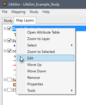
 Add new features (A)
 Insert vertex (I)
 Break line feature into two... (K)
 Continue from end (lines only)
 Add new line or polygon to existing feature
 Feature Snapping Settings
 Undo (Ctrl + Z)
 Redo (Ctrl + Y)
 Save Edits (Ctrl + S)
 Stop Editing
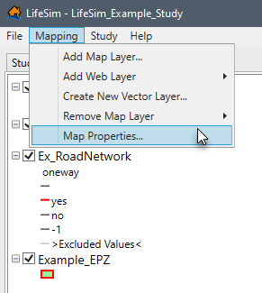
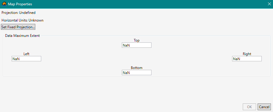
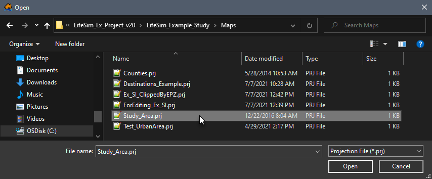
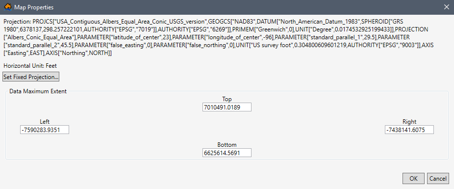
 ) layers
in the Map Layers tab will display in the map window (Figure). The user can turn map layers
on or off, adjust the properties of the layers, and modify the order of the layers for viewing in the map window.
) layers
in the Map Layers tab will display in the map window (Figure). The user can turn map layers
on or off, adjust the properties of the layers, and modify the order of the layers for viewing in the map window.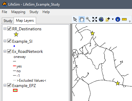
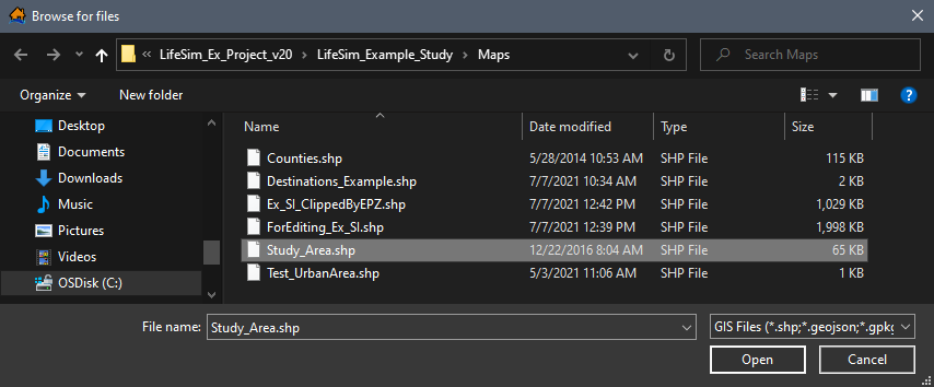
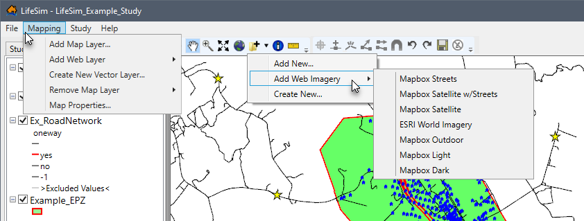
 , that map layer
will automatically be added to the bottom of the Map Layer Tree and will be underneath all layers listed above the internet map. At times, it may be
desirable to have various
map layers drawn in a different order in the map window.
, that map layer
will automatically be added to the bottom of the Map Layer Tree and will be underneath all layers listed above the internet map. At times, it may be
desirable to have various
map layers drawn in a different order in the map window.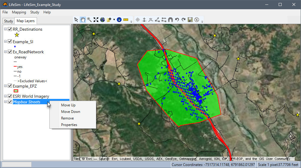
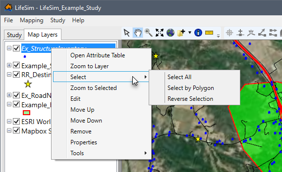
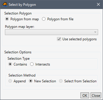
 . The Select a Polygon Shapefile browser will open. The user will need to navigate to the file of choice and select the desired polygon shapefile (*.shp). Click Open, the Select a Polygon Shapefile browser will close, and the name of the selected polygon shapefile will display in the Polygon shapefile box (Figure).
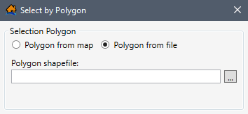
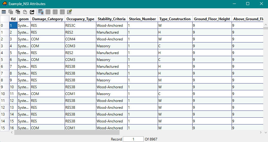
 Select all cells
 Copy Selected Cells
 Copy Selected Cells with Table Headers
 Paste from the Clipboard into the Table
 Export Table
 Start Feature Edit Session: enables
editing for the map layer open in the attributes table. For more information regarding editing map layers
and map layer attributes, review Editing Map Layer Features and
Attributes and Editing in the Attribute
Table respectively.
Start Feature Edit Session: enables
editing for the map layer open in the attributes table. For more information regarding editing map layers
and map layer attributes, review Editing Map Layer Features and
Attributes and Editing in the Attribute
Table respectively. Select Rows By Attribute
 Show All Rows
 Show Selected Rows Only
 Deselect All Rows
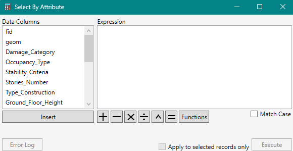
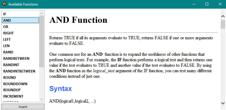
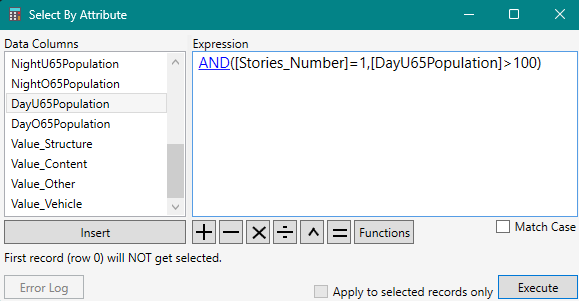
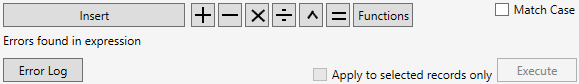
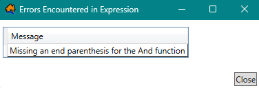
 and Deselect All Rows
  icons are now active.
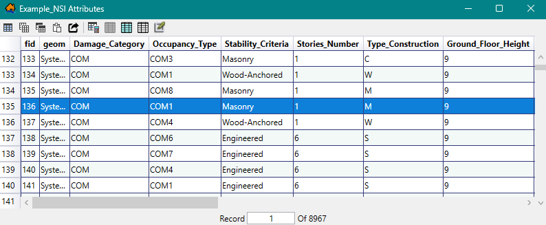
 (as opposed to the original blue
  color). Double-clicking in the map window will deselect the features.
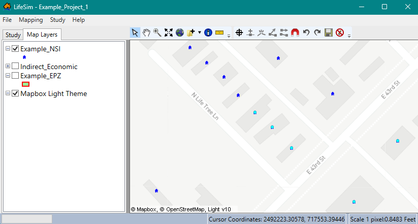
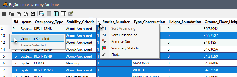
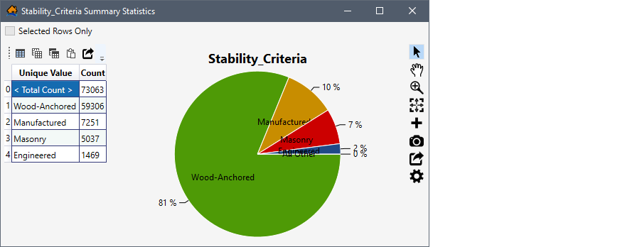
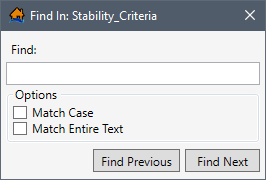
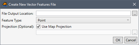
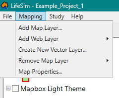
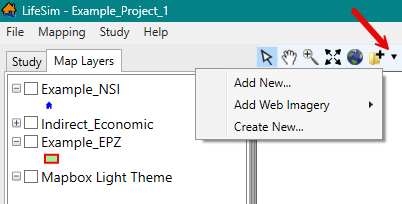
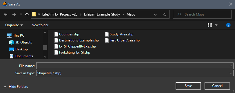
 Point: Features that are too small to be represented by lines or polygons. Examples include structure inventories and destinations.
 Polyline: Features that represent the shape and location of geographic objects, such as the road networks.
 Polygon: A set of many-sided area features which represent the shape and location of a feature or set of features, such as emergency planning zone(s).
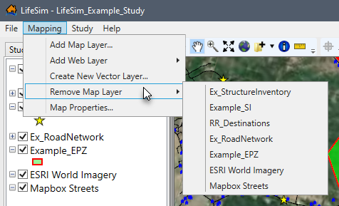
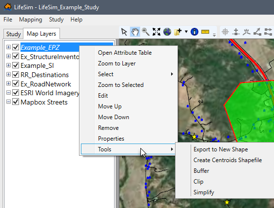
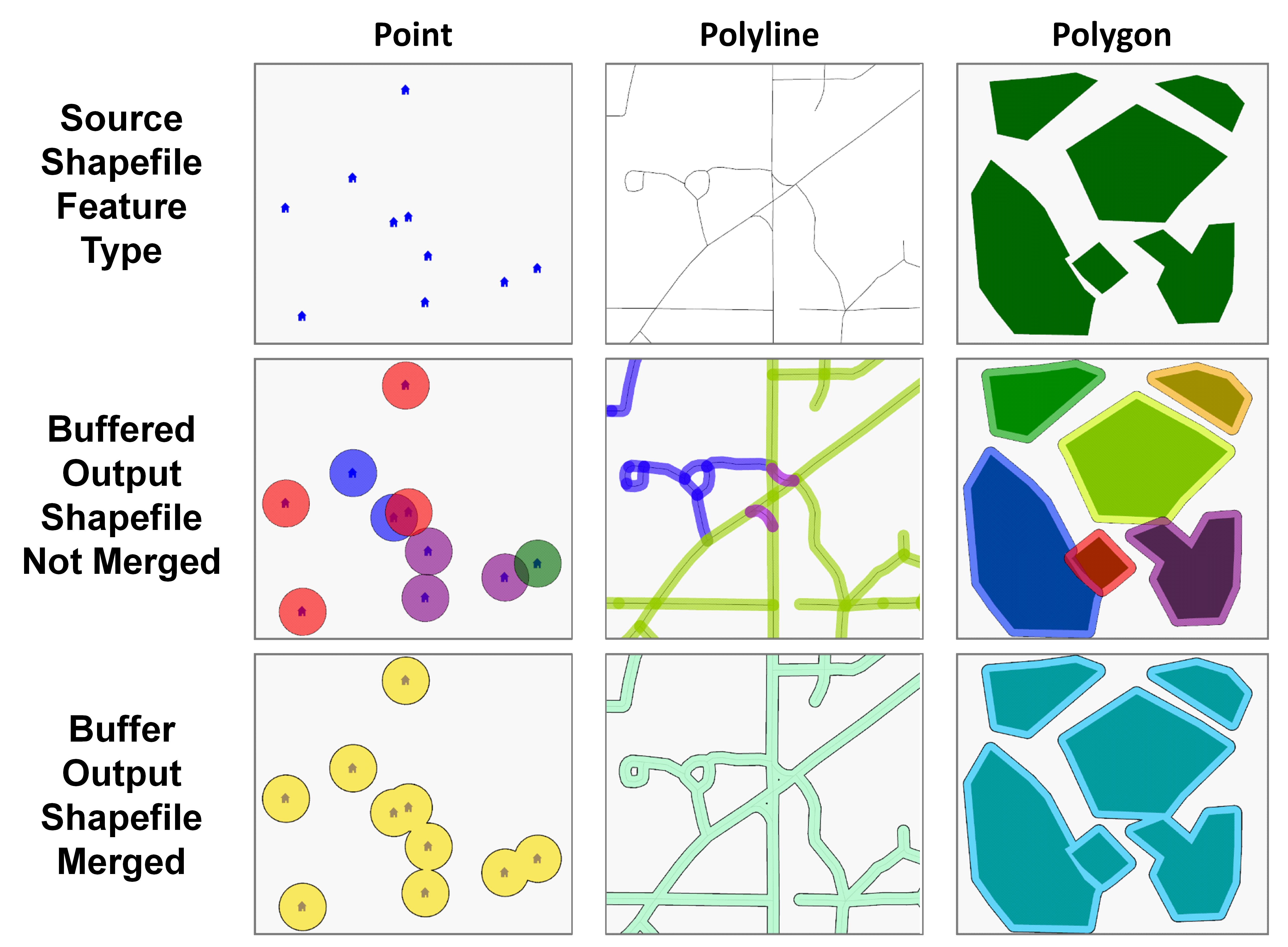
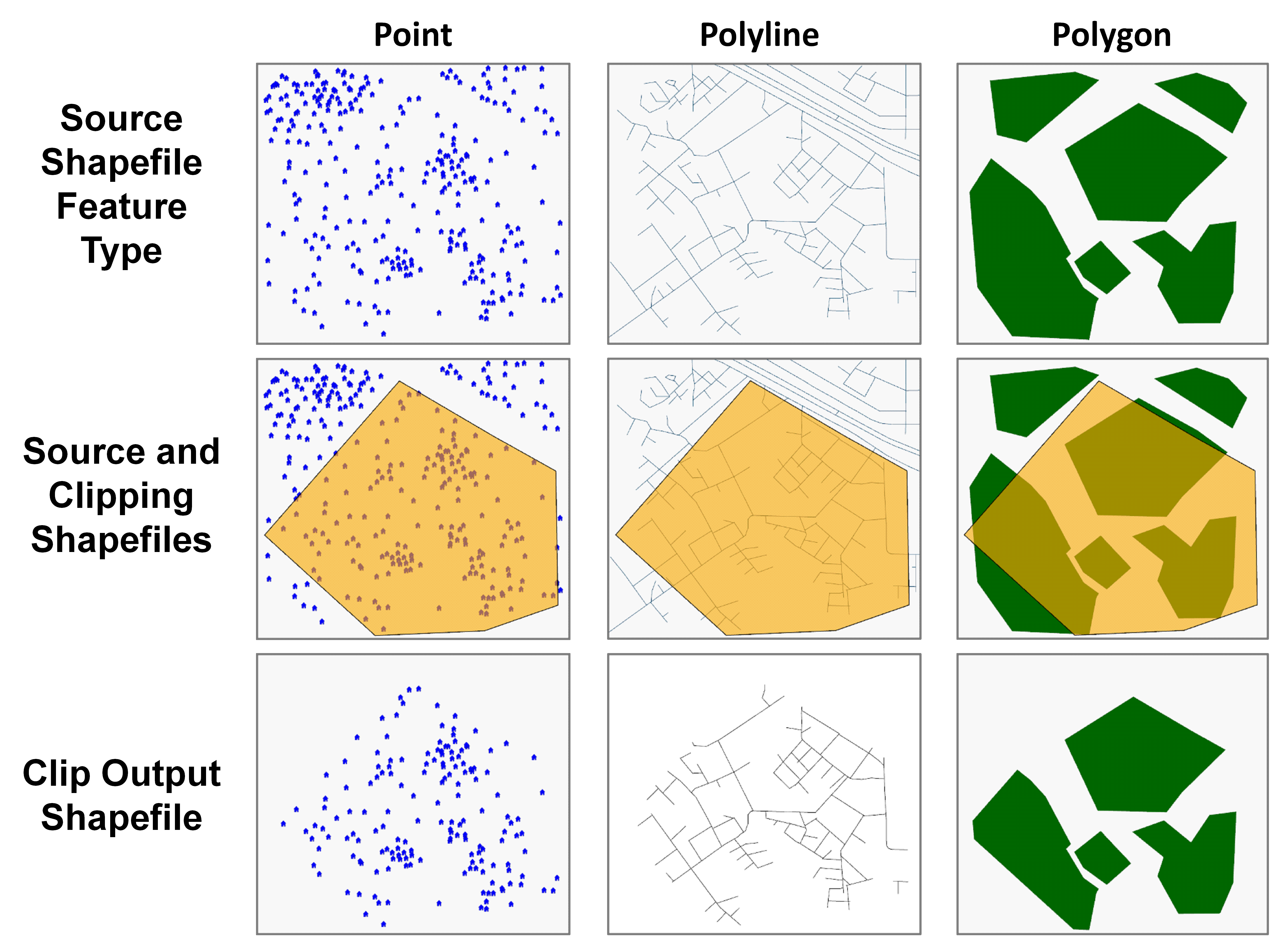
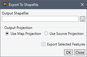
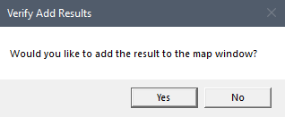
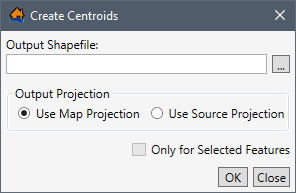
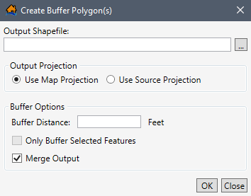
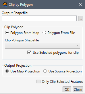
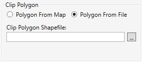
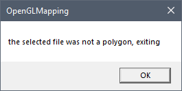
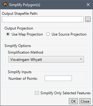
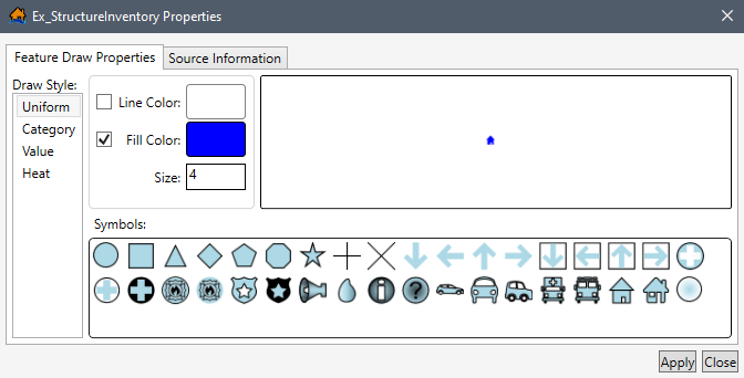
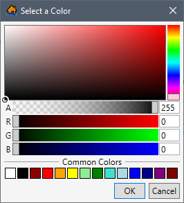
 white-black circle in the Color Bar display area. This circle shows the location of the selected color. Click anywhere inside the Color Pallet area, and the white circle will be moved to the new location and the Color Properties values will change automatically.
 Bright Red: Red 255, Green 0, Blue 0
 White: Red 255, Green 255, Blue 255
 Bright Yellow: Red 255, Green 255, Blue 0
 Bright Teal: Red 0, Green 255, Blue 255
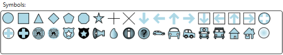
 Line Color. Then, click the Line Color preview box. The Select a Color dialog box will open (Figure).
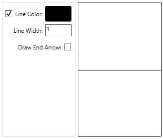
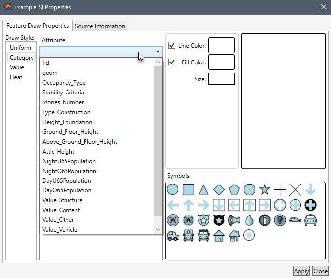
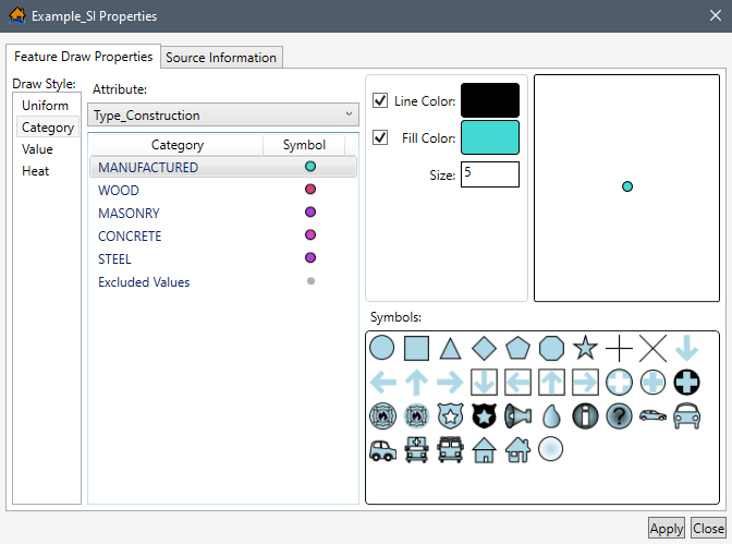
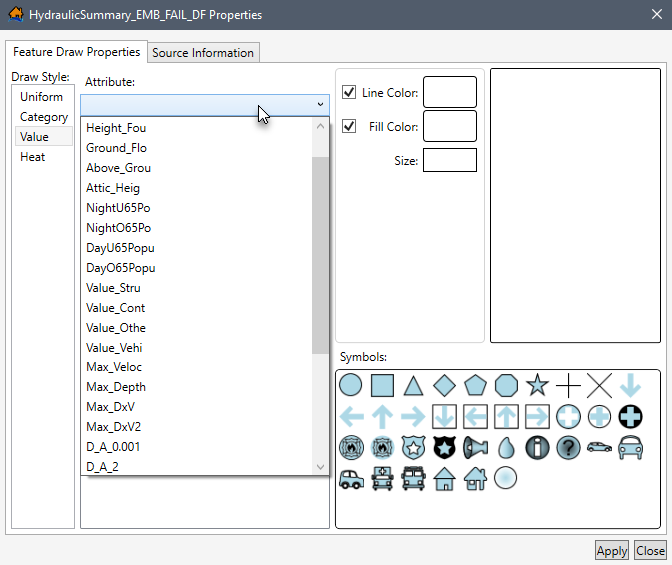
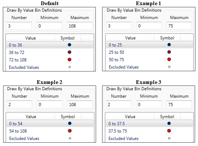
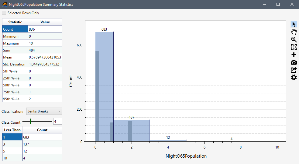
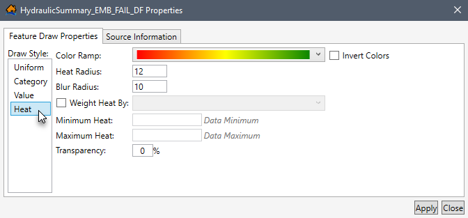
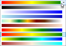
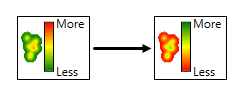
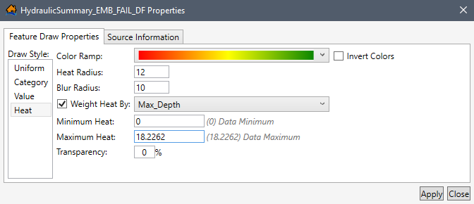
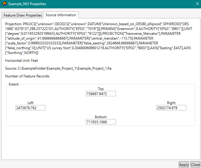
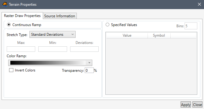
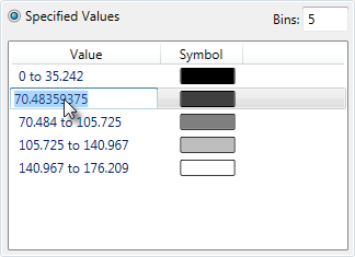
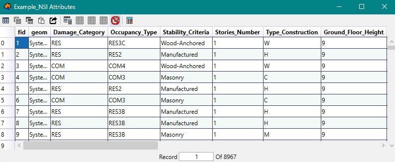
 Open Field Calculator
 Stop Feature Edit Session
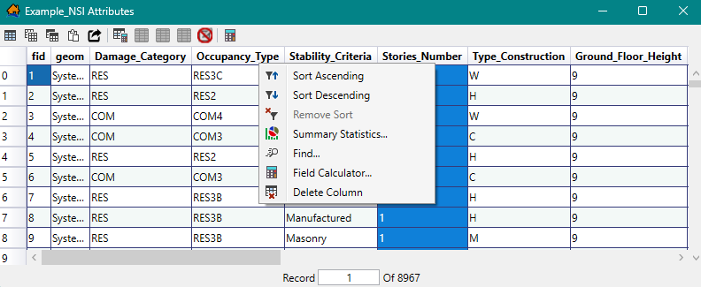
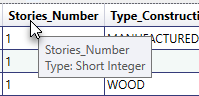
 Delete Column
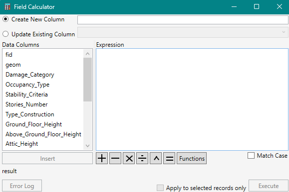
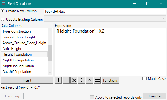
 from the Editor Toolbar.
 button from
the Editor Toolbar.
button from
the Editor Toolbar.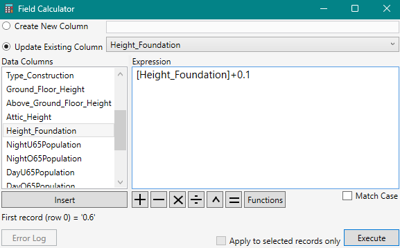
 button will then become active, and the user can redo the change made to the field.
 (note the dot in the center of the cursor). Click inside the map window and new points will be placed at the center of the cross-hairs (where the dot is located). Review Editing Point Map Layers for more information on added or editing point features. Click
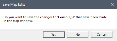
 . Then, click on the feature to be moved or click + hold + drag a rectangle around the feature(s). With the point selected, click and drag the point to the desired location (Figure). The user can move also multiple points at once.

 . The cursor will change to
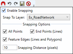
 star symbol. The properties for the newly created destinations map layer (e.g., Example_Destinations) can be modified from the default general point layer symbol. Alternatively, users can modify the map layer properties before adding any new points to the newly created map layer.