LifeSim Interface
The LifeSim interface allows users to enter data, review data, create alternatives, run simulations, and review results.
Main Window
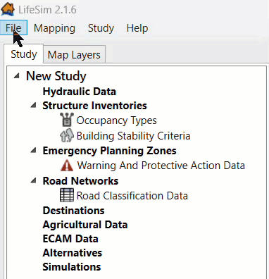
The main window (also described in section Installing and Starting LifeSim) displays the framework for the LifeSim software (Figure).
.png)
The main window is organized with a Title Bar, a Menu Bar, two tabs (Study and Map Layers), a Map Window (with an associated toolbar), and the Status Bar. The following describes basic elements of the main window:
Title Bar: Displays the Version number (Version 2.1.6), for Version 2.0 and above, and the name of the active LifeSim study.
Menu Bar: Contains the LifeSim menus.
Study and Map Layers Tabs
- The Study tab contains a Study Tree that guides users when adding the building blocks of a LifeSim study.
- The Map Layers tab contains a list of all map layers that are currently part of the active study. Clicking a tab opens the tab specific information and commands.
Map Window: Used to graphically display the LifeSim study components and imported map layers, which are geographically referenced (geo-referenced).
Map Toolbar: Contains tools used to setup, navigate, and edit within the LifeSim map window.
Status Bar: Displays messages related to incoming data and status of the LifeSim software for informational purposes.
Menu Bar
The menu bar (Figure) of LifeSim provides the user with many commands to perform various functions. An overview for each menu in LifeSim software is provided.
File: The File menu allows the user to perform study management functions such as creating, opening, closing, and saving an LifeSim study.
- Available commands are: Create New, Open Existing, Save, Save As, Zip Project, Compress Project, and Exit.
- This menu also displays a list of previously opened LifeSim studies and selecting one automatically opens the selected study.
Mapping: From the Mapping menu, users can add or remove map layers from the Map Layers tab, shown in the map window.
- Available commands are: Add Map Layer, Add Web Layer, Create New Vector Layer, Remove Map Layer, and Map Properties.
- Map layers that can be added to a LifeSim study are: *.shp, *.flt, *.tif, and *.vrt, or Web Imagery layers.
- Other available functions from the Mapping menu are creating vector layers and modifying or importing map projections.
Study: From the Study menu, users can import, create, modify, and edit the building blocks of a LifeSim study.
- Available commands are: Hydraulic Data, Structure Inventories, Emergency Planning Data, Road Network Data, Destinations Data, Agricultural Crop Data, ECAM Data, Alternatives, and Simulations.
Help: Directs user to the current version of the LifeSim User's Guide; and information about LifeSim.
Tabs
The LifeSim main window is organized into two tabs (Figure) that allow the user to view, enter, and edit LifeSim study data or to view and manipulate any map layer geographically in the map window.
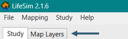
Study Tab: Allows a user to view, add, and edit data; and add/remove map layers for a LifeSim study. The Study tab is the default tab and provides a view of the study data in a tree (Study Tree). From the Study Tree, a user can create, edit, and delete datasets, alternatives and simulations.
The Study Tree lists datasets, alternatives and simulations that have been created.
Map Layers Tab: The Map Layers tab provides a list of the map layers in a tree (Map Layers Tree). From the Map Layers tab, a user can import, create, edit and delete map layers. The Map Layers Tree allows users to also display map layers in the map window. However, only selected layers in the Map Layers tab will display in the map window.
The user can turn map layers on or off, adjust the properties of the layers, modify the order of the layers for viewing in the map window. Appendix B provides greater detail on the Map Layers tab and associated map window.
Map Window
The Map Window in LifeSim provides a way to graphically display LifeSim components. This section is designed to give a brief overview of what is available in the map window and map layers. For more detail on the mapping functionality in LifeSim, refer to Appendix B.
The Map Toolbar contains two sets of tools (Figure): General Toolbar and Editor Toolbar.

If a tool has a parenthesis after the tooltip, the letter in the parentheses represents a hot key that allows a user to access the tool
through the keyboard. For example, to access
the  Query Features Tool (Q)
through keyboard selections, the user will click the Shift + Q keys while over the Map Window. This will activate the Query Features Tool.
A list of all of the hot keys is located in Appendix B.
Query Features Tool (Q)
through keyboard selections, the user will click the Shift + Q keys while over the Map Window. This will activate the Query Features Tool.
A list of all of the hot keys is located in Appendix B.
General Toolbar
The General Toolbar includes the Select Tool (B), Pan Tool (P), Fixed Zoom Out Tool (O), Zoom In Tool (Z), Zoom to full extents, Add Data, Query Features Tool (Q), and Measure Distance Tool (M). These tools change the appearance of the cursor, as well as the functionality of the mouse cursor in the map window. Table describes each tool's functionality.
| Tool | Functionality |
|---|---|
 Select Tool (B) Select Tool (B) | Select elements displayed in the Map Window. To select features, click on a feature or click, hold, and drag a rectangle around features to select them in the Map Window. Additionally, the Select tool allows users to access shortcut menus which can be customized when in editing mode. Refer to Appendix B for more information regarding editing mode. |
 Pan Tool (P) Pan Tool (P) | Pan the Map Window; click the Pan tool and click, hold and move the mouse around the Map Window. Also, if the mouse has a wheel, then the user can pan the Map Window by using the wheel (click and hold the wheel to pan). |
 Zoom In Tool (Z) Zoom In Tool (Z) | Zoom in to areas of the Map Window. To zoom in, hold the mouse button down and outline the area of interest to enlarge. Also, if the mouse has a wheel, then the user can zoom in or out using the wheel (wheel up zooms in and wheel down zooms out). |
 Fixed Zoom Out Tool (O) Fixed Zoom Out Tool (O) | Zooms out to a fixed distance. Click the Fixed Zoom Out tool once and the Map Window view will zoom out a fixed distance. Double-click on the tool icon, and the Map Window view will zoom out twice the fixed distance. Additionally, the user can utilize the shortcut menu option: right-click anywhere in the Map Window to zoom in or out a fixed distance. |
 Zoom to full extents Zoom to full extents | A quick way to re-center the map by zooming out to the full geographical extent of the map layers in the Map Window. Web layers do not affect the map extents. |
 Add Data Add Data | After clicking the Add Data tool, the File Explorer browser window will open. This browser allows users to navigate to layers (including *.shp, *.flt, *.tif, and *.vrt) of interest and add the layer(s) to the map window. If the user clicks the down arrow next to the Add Data tool, a shortcut menu will appear which allows the user to Add New [Data], Add Web Imagery, or Create New [Vector Features File] that is added to the Map Window. |
| Query Features Tool (Q) | Identifies the geographic feature or place currently selected in the Map Window. Alternatively, multiple features can be identified by dragging a box over the desired area. Once a selection is made, the Feature Query dialog box will open with the information presented in table format separated by Feature type. Only visible layers in the Map Window will be queried. |
 Measure Distance Tool (M) Measure Distance Tool (M) | Measure the distance along a specified line. With the tool selected, click to initiate the measure line. Each subsequent click will add a new point to the measure line. When finished, double-click on the location of the final point. The Measure Results dialog box will open and display the distance in the units the user has chosen (feet, miles, meters, or kilometers). |
Editor Toolbar
The set of tools located in the Editor Toolbar initiate an editing session for the selected layer. When a user right-clicks on a map layer in the Map Layers tab, from the shortcut menu (Figure), click Edit, and the tools in the Editor Toolbar become active. Only one map layer can be edited at one time.
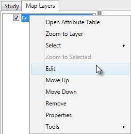
For lines and polygons, there are two editing modes: feature edit and vertex edit. Clicking on a selected feature puts the user into the feature edit mode (move, delete, reverse). Double-clicking on a selected feature puts the user in the vertex edit mode (add, delete, edit vertex points). Refer to Appendix B for demonstration on both modes.
There are some tools available during an edit session which are not available from the shortcut menu (Figure) or the Editor Toolbar.
- Clicking Delete will delete all currently selected features or currently selected vertices, depending on which mode the user is in.
- Clicking the R key will reverse the direction of a currently selected line feature.
- Right-clicking during an edit session allows the user to do multiple tasks depending on what is clicked.
Detailed information on all of the functionality of the editing tools is available in Appendix B. The following is the functionality of each Editor Toolbar tool.
| Tool | Functionality |
|---|---|
 Add new features (A) Add new features (A) | Add a new feature to the editable map layer by left-clicking to add feature data. Selected features can be deleted by either clicking the Delete key, or right-click on the selected feature(s) and from the shortcut menu, click Delete Selected Features. |
 Insert vertex (I) Insert vertex (I) | Add a vertex to an existing line or polygon map layer. The tool becomes available when the selected feature is in vertex edit mode. As the cursor gets close to the line or polygon edge, the Map Window will display what the updated feature will look like if a vertex is added at the cursor. Left-click to insert the new vertex. |
 Break line feature into two... (K) Break line feature into two... (K) | Split a line feature into two features at the point the user clicked on the line. The user needs to be in the feature edit mode for this tool to be enabled. |
 Continue from end (lines only) Continue from end (lines only) | Continue a line feature from the end point of the line feature to the point to a second point clicked in the Map Window. Double-click to finish the line continuation edits or right-click and choose Finish Editing Vertices or choose a different tool to finish the line continuation. The user needs to be in the vertex edit mode for this tool to be enabled. |
 Add new line or polygon to existing feature Add new line or polygon to existing feature | Add a polygon or line to an existing selected polygon or line feature. For example, to add a hole to a polygon, click to add points defining the hole and double-click to finish. The user needs to be in the vertex edit mode for this tool to be enabled. |
 Feature Snapping Settings Feature Snapping Settings | Define snapping rules when editing. Snapping will automatically move the desired action to the nearest snap point when the cursor is close. This can be very useful when trying to line up endpoints of line features or place points directly on top of other features. Enable snapping by clicking Enable Snapping. From the Snap to Layer list, select the desired feature to snap to, then select under Snapping Options how snapping will be applied (to all points, end points, or edges). |
 Undo (Ctrl + Z) Undo (Ctrl + Z) | Undo changes made during an edit session. Only enabled if there are edits that can be undone. |
 Redo (Ctrl + Y) Redo (Ctrl + Y) | Redo changes made. Only enabled if there are edits to redo. |
 Save Edits (Ctrl + S) Save Edits (Ctrl + S) | Saves all edits made during the editing session. Only enabled if edits have been made. |
 Stop Editing Stop Editing | Stops the edit session. At this point a new map layer can be selected for editing. If edits have been made, then the user will be prompted to save them before stopping the edit session. |
Table Tools
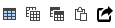
Several tables in LifeSim contain the Export and Copy Tools (Figure) and the Selection Tools (Figure) toolbars.

For example, the Simulation Results Tables (Figure) includes the Export and Copy Tools and the Selection Tools toolbars.
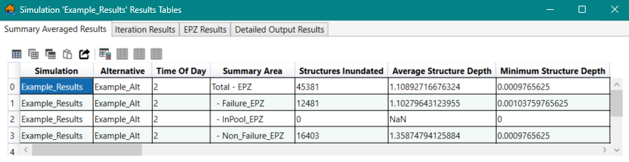
For additional information on viewing LifeSim results, review Simulation Results Table.
Export and Copy Tools
Table describes the functionality of the Export and Copy Tools toolbar.
| Tool | Functionality |
|---|---|
 Select all cells Select all cells | Selects all cells in the table. |
 Copy Selected Cells Copy Selected Cells | Copies cells selected in the table. The information is copied to the clipboard and needs to be pasted to another application (e.g., Microsoft Excel®) for saving. |
 Copy Selected Cells with Table Headers Copy Selected Cells with Table Headers | Copies cells selected in the table and the table headers. The information is copied to the clipboard and needs to be pasted to another application (e.g., Microsoft Excel®) for saving. |
 Paste from the Clipboard into the Table Paste from the Clipboard into the Table | Pastes data copied from another table into the current table. |
 Export Table Export Table | Opens a Save As browser window (Figure), which allows the user to export the data in the table to a Microsoft Excel® (*.xlsx) file. |

Selection Tools
Table describes the functionality of the Selection Tools toolbar.
| Tool | Functionality |
|---|---|
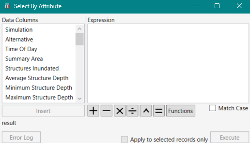
 Select Rows By Attribute Select Rows By Attribute | Opens the Select By Attribute dialog box (Figure), which allows the user to perform queries, make selections, and locate features in the table. |
 Show All Rows Show All Rows | Display all rows (selected or unselected) in the table. |
 Show Selected Rows Only Show Selected Rows Only | Only display features selected in the table. |
 Deselect All Rows Deselect All Rows | Unselects all rows which were selected in the table. |
Customizing Plots and Plotting Tools
Several plots include the General Plotting Tools. For example, the Time Series Data plotting window shown below (included in the Hydraulic Data importers, as described in Hydraulic Data Import Options) includes the General Plotting Tools.
General Plotting Tools
Through the use of the General Plotting Tools, plots are highly customizable and offer an array of information to assist in reviewing the data, such as the time series data plot in Figure. The following are the available plotting tools and their functionality (Table).
| Tool | Functionality |
|---|---|
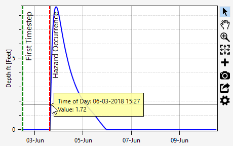
 Track Data Track Data | Using the Track Data tool, click and hold inside the plot window. A yellow callout box will display that provides the data at the specific x and y location (Figure). For example, in Figure, the callout displays the Time of Day and corresponding Value for the specified location along the hydrograph. Click and drag to get information in a yellow callout box anywhere along the graph. |
 Pan Pan | Pan the plot window. To pan, click and hold while moving the mouse. Another way to pan is press down on the scroll wheel (middle mouse button) of the mouse (if the mouse has a scroll wheel). |
 Zoom In Zoom In | Zoom in to areas of the Map Window. To zoom in, hold the mouse button down and outline the area of interest to enlarge. Also, if the mouse has a wheel, then the user can zoom in or out using the wheel (wheel up zooms in and wheel down zooms out). |
| Zoom Full Extents | A quick way to re-center the data displayed in the plot window by zooming out to the full extent of the plot. |
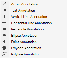
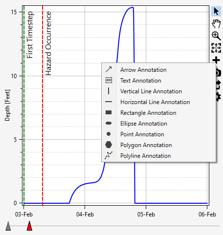
 Add Annotation Add Annotation | Opens a list of annotations (Figure) that can be added to the plot. Three annotation types are available. To add the first type (Text, Vertical Line, Horizontal Line and Point), simply click and drag to the desired location. To add the second type (Arrow, Rectangle, and Ellipse), click, drag and release. To add the third type, click a starting point, additional clicks continue the polyline or polygon, and double-click to complete the polyline or polygon annotation. Edit the default text for the added annotation by double-clicking to select the text and enter. Default annotation properties can be modified using the Plot Properties
 tool.
NOTE: the Save Plot Image tool.
NOTE: the Save Plot Image  tool will include all annotations added to the time series plot. tool will include all annotations added to the time series plot. |
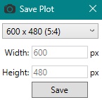
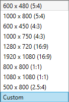
| Save Plot Image | Save the data displayed in the plot window. The Save Plot Image tool opens the Save Plot dialog box (Figure). From the Save Plot dialog, select from default pixel (px) width and height of the plot or set a custom size (Figure). Click Save. A Save As browser window will open. Navigate to the location (directory) to save the plot, enter a name (required) in the File name box, and select the file type from the available options (*.png,*.pdf, *.svg). Click Save, and the Save As browser will close.
NOTE: the Save Plot Image tool will include all annotations added to the time series plot and all alterations made to the plot using the Plot Properties
tool. |
| Export Series Data | Opens a Save As browser window, which allows the user to export the data as a comma delimited (*.csv), a Microsoft Excel® (*.xlsx) or Sqlite (*.sqlite) file. |
| Plot Properties | Configure default properties for customizing LifeSim plot window. For example, the Time Series Data plot (Figure) can be customized by clicking the Plot Properties tool to open the Plot Properties dialog box (Figure). Customizing Plots Overview provides a detailed explanation regarding customizing plots in LifeSim. |
Figures associated with General Plotting Tools, mentioned in Table, are shown below.
Customizing Plots Overview
Various attributes of a plot can be customized by clicking the Plot Properties
tool or right clicking on a plot
and selecting an edit option, from specific plot windows.
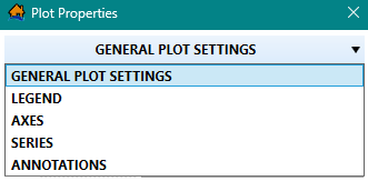
The Plot Properties dialog will open and allow the user to configure multiple display properties for the individual plot. Access different customization editors by toggling through the plot properties dropdown menu to access the different editing options (Figure). The five dropdown editing options (GENERAL PLOT SETTINGS, LEGEND, AXES, SERIES, and ANNOTATIONS) are described in the subsequent sections.
Depending on the plot properties dropdown menu selection, the Plot Properties dialog updates to include a selector
dropdown menu and expandable sections. For example, the AXES (Figure) editor
includes a dropdown menu to allow users to select the x- or y-axis and also contains three tabs for editing the general, labels, or grid lines.
Collapse the section by clicking the expand  button,
or click the section
button,
or click the section
 arrow to expand the section.
Depending on the expanded editing section, users can enter text labels, choose the color, and/or use dropdown menus to modify the size, type, weight,
padding, and/or alignment of the specified component of the plot. In general, checkboxes (  or
or
 ) allow users to turn on or off the
display of an item (e.g., turn on or off the visibility of the legend from the LEGEND AREA section displayed in
Figure).
) allow users to turn on or off the
display of an item (e.g., turn on or off the visibility of the legend from the LEGEND AREA section displayed in
Figure).
Once customization of the plot properties has been completed, click the Close  dialog
button (Figure).
dialog
button (Figure).
To edit the default color selection, click any color box (e.g., Color, Plot Area Color, Border Color, Background Color, etc.) to open a color chooser window (Figure).
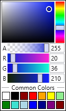
The color chooser window provides:
- A large color picker box (tint varies along the left axis, tone varies along the right axis, and saturation varies along the top axis).
- A vertical color hue slider bar.
- A transparency horizontal slider bar.
- A Common Colors section that provides several default color swatches.
Use the vertical hue slider bar to select a color (e.g., blue in Figure) and use the color picker box to choose the desired shade, tint and tone (adding black, white and gray respectively) for the chosen color. Selecting a color in the color chooser window automatically updates the color box in Plot Properties dialog.
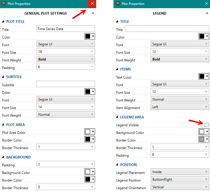
GENERAL PLOT SETTINGS
By default, the Plot Properties dialog opens with the GENERAL PLOT SETTINGS (Figure) selected from the dropdown menu. Options for modifying the plot general settings include:
- Plot title.
- Subtitle.
- Plot area.
- Background.
LEGEND
To modify the legend properties, select LEGEND from the Plot Properties dropdown menu (Figure).
Users can modify:
- Title
- Items
- Legend Area
- Position
NOTE: if making modifications to the legend, make sure the Legend Visible
(Figure)
checkbox is checked
or the legend will not
display in the plot window.
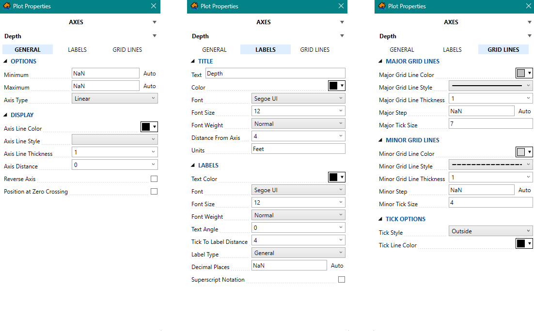
AXES
To edit the plot axes, select AXES from the Plot Properties dropdown menu (Figure). When modifying the plot axes, choose the axis (e.g., Y Values in Figure) and the component to modify (GENERAL, LABELS, or GRID LINES tab). From the GENERAL tab, modify the axis minimum, maximum, axis type, or axis display properties. From the LABELS tab, edit the axis label, text color, font, distance from the axis and/or enter the units for the axis. From the GRID LINES tab, modify the major and minor grid lines and the tick mark options.
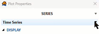
SERIES
The data series curves can be modified by selecting SERIES from the Plot Properties dropdown menu (Figure). Users can select the specific data series in the plot (e.g., Time Series in Figure) when more than one data series is displayed in a plot window. Users can modify the series display and markers (if applicable). For example, if the series is a time series hydrograph, then the display and marker sections are available to modify the line and marker style, color, thickness and size can be modified. However, if the series is box and whisker, then only the display section is available to modify the box and line style, color, thickness and size can be modified.
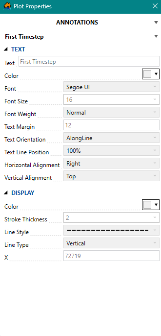
ANNOTATIONS
To add annotations, from the Plot Properties dropdown menu, select ANNOTATIONS (Figure). Depending on the plot, default annotations will already be added to the plot. For the example provided in Figure, the default annotations included in the time series hydrograph are the First Timestep (green vertical dashed line with text) and Hazard Occurrence (red vertical dashed line with label).
Users can modify the text and display properties of existing or added annotations. For the example provided in Figure, the First Timestep annotation is selected from the annotation dropdown menu and the TEXT and DISPLAY sections are expanded to display the default First Timestep annotation properties.
Add an additional annotation to the plot by selecting the Add Annotation tool (Figure).
Annotation types include arrow, text, line, rectangle, ellipse, point, polygon, or polyline. Users also have the option to remove added annotations
(including default annotations) by clicking the Delete Annotation
 button.
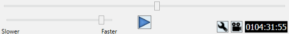
Animation Toolbar
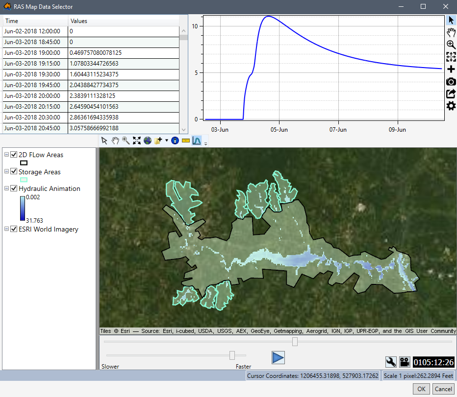
When animations are viewed in the Map Window, an Animation Toolbar (Figure) appears. For example, from the RAS Map Data Selector dialog box (Figure), users can import hydraulic data from a RAS map. Another example is when users view hydraulic or evacuation animations results in the Map Window (refer to View Result Map in the Map Window).
From the Animation Toolbar at the bottom of the RAS Map Data Selector (Figure), the
user can view (animate) the HEC-RAS depth simulation for the specified plan. The controls for the animation bar function the same as the controls to
a video player. Use the slider bars to modify the speed (faster or slower) and position of the animation playback. To modify the animation settings,
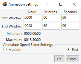
click  , and the Animation
Settings dialog box (Figure) opens.
, and the Animation
Settings dialog box (Figure) opens.
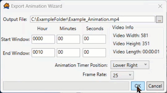
The user can export a copy of the animation.
Click
 , and the Export Animation
Wizard opens. To save an animation output file, click
, and the Export Animation
Wizard opens. To save an animation output file, click
 ,
navigate to the location (directory) to save the animation, enter a name (required) in the File
name box, and verify the file type from the available options (*.mp4, *.wmv). Click Save, and the
Save As browser will close.
,
navigate to the location (directory) to save the animation, enter a name (required) in the File
name box, and verify the file type from the available options (*.mp4, *.wmv). Click Save, and the
Save As browser will close.
From the Export Animation Wizard, set the desired Start Window and End Window, Animation Timer Position, and Frame Rate. To complete the export, click OK. The progress bar at the bottom of the Export Animation Wizard provides the progress of creating the video file (Figure). Once complete, the Export Animation Wizard closes.