LifeSim

Consequences

Chapter Overview

This chapter covers how consequences are calculated in LifeSim. Consequences may be life loss, direct economic damages (e.g., property, agriculture), or indirect economic damages. Computational Procedure described how LifeSim calculations re-distribute the initial population by evacuation group through emergency response to avoid the oncoming hazard. They may have evacuated vertically in their structure or evacuated the structure by vehicle or on foot. The result of those calculations places each evacuating group in a final location: safe, no hazard, low hazard, or high hazard. In this chapter, the impact of the hydraulic conditions is considered for each person and evacuating group to determine direct life loss. In addition, the hydraulic conditions at each structure and agricultural field are used to determine direct and indirect economic damages.

Life Loss

Based on the assigned hazard zone categories, life-loss estimates are made using life-loss probability distributions developed by McClelland and Bowles (2000) [?], updated by Aboelata, Bowles, and McClelland (2003) [?], Aboelata and Bowles (2008) [?], and revised by USACE (Fatality Rates).

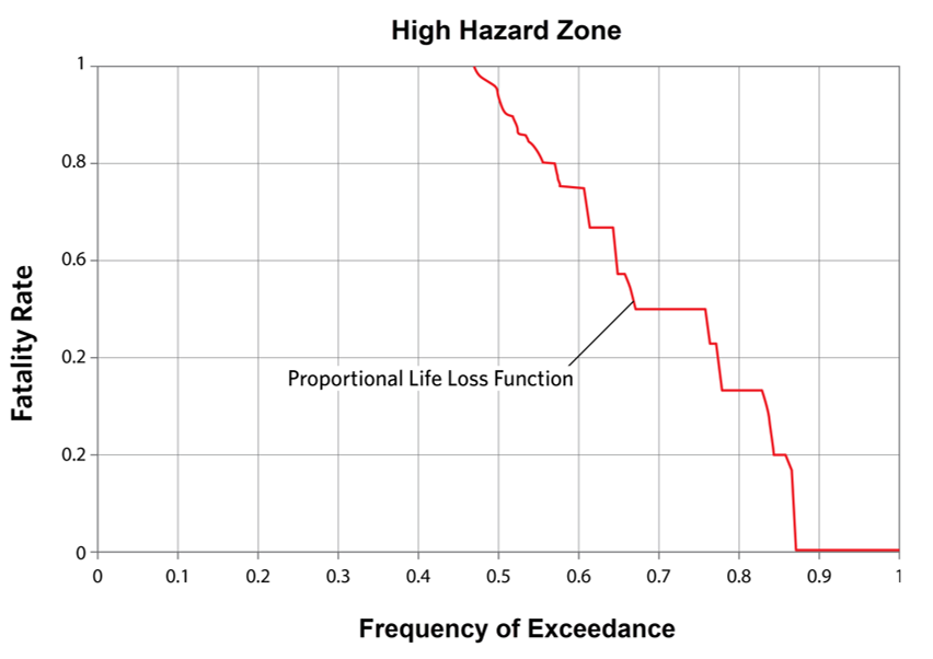
Figure shows the distribution of fatality rates for population groups in the high hazard zone.

As described in Population Parameters, the population is categorized as being in either a low or high hazard zone. LifeSim can calculate life loss for each person that ends up in either a low hazard or high hazard zone. The overall calculation is the same for both zones; only the hazard zone function (Figure) is different. For each group that has been assigned to a zone, a fatality rate is acquired by randomly sampling the relative frequency of exceedance. In other words, a group in the high hazard zone can be in a scenario representative of any other group represented in the dataset. By sampling the frequency of exceedance, naturally variable occurrences such as being able to hang on to passing debris or finding an air pocket in a submerged structure are expressed.

Figure provides an example for one evacuating group. Assume the evacuating group consists of three people in a structure, and the structure loses stability. In this example, the evacuating group is considered in the high hazard zone and randomly assigned a relative frequency of exceedance between zero and one (assume 0.58). That value on the x-axis translates to a fatality rate on the y-axis of 0.75. The fatality rate represents, on average, 75% of the evacuating group will lose their life.

Figure: High hazard fatality rate function used in LifeSim.

Figure: Example sampling of high hazard fatality rate function for one evacuating group.

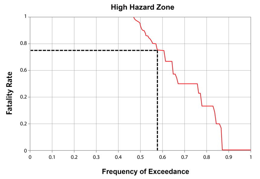
After the fatality rate is determined, life loss is calculated for each person in the group. To determine individual fatality, each person in the group samples a random value between 0 and 1. If the random number is above 0.75, then the person survives. If it is below 0.75, then the person does not. In the example case, the structure fails, so all three people are placed in the high hazard zone. However, evacuating groups in flooded structures that do not collapse may be split between low and high hazard zones based on age and/or mobility.

To reiterate the process, sample one fatality rate per group from either the high or low hazard function, then sample fatality per person in the group. By sampling the hazard zone fatality rate function randomly for each evacuating group, the fatality rates sampled for all the evacuating groups in the population define the shape of the function. For example, about 47% of evacuating groups will have 100% fatalities in their group and around 13% of evacuating groups will have no fatalities in the group. The remaining 40% of the groups have some chance of fatalities and survival defined by the function.

The reason for applying fatality rates at the level of the evacuating group is that conditions are fairly consistent for a group. This reason is why the data to support the functions was collected at a group level. Research suggests that members of an evacuating group impact each other's chances of survival in complex ways that are not modeled. By capturing these hidden dynamics in the data set and applying them at the evacuating group level, LifeSim more accurately replicates the factors leading to life loss. For example, in a family with young children, the adults will assist the children to reach safety and be hindered themselves by providing assistance. In a group of capable adults, the overall risk may be reduced by cooperation versus each person considered on their own.

Property Damage

Structure, Content, Vehicle, and Other Damage

Direct damages to a building, its contents, and its vehicles are calculated for a single structure as follows:

$$D = d_s * v_s + d_c * v_c + d_v * v_v + d_o * v_o$$

where

D = total direct damage for a structure.
_s = structure.
_c = contents.
_v = vehicles.
_o = other.
d = damage (in percent) as a function of depth and depth-damage function.
v = property value.

To determine the percent direct damage to buildings, contents, and vehicles, both the depth at the structure and occupancy type of the structure need to be known. The depth is considered the maximum depth at the structure minus the foundation height. The occupancy type is specified as part of the structure inventory and is associated with three individual depth-percent damage relationships, one each for the building, contents, and vehicles. There is also the option to define a fourth depth-percent damage function for an additional "other" category. Therefore, the depth at the structure can be used to determine the percentage that the three components of the structure are damaged. This percent damage can then be multiplied by the building, contents, and vehicles values (specified in the structure inventory) to determine the total direct damage that occurs at and within a structure.

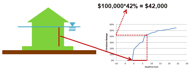
A schematic of the direct damage computation procedure for a building is shown in Figure. At a depth of 7 feet, the building is 42% damaged based on the depth-damage relationship. Multiplying the building value (100,000 USD) by the damage (42%) results in a direct building damage of 42,000 USD. The direct damage to the contents and vehicles will also need to be added to the building damage of 42,000 USD to determine the total damage at and within the structure.

Figure: Direct building damage calculation procedure.

Damages to vehicles are not impacted by the number of vehicles that leave during an evacuation. That consideration must be made outside of LifeSim before updating the structure inventory. The reason for not reducing the number of cars is that there are currently no good approximations for the number of cars at each structure. Since the population shifts according to work and school considerations, the location of the car may not match the population.

The second consideration that can impact the direct damage computations occurs when a structure's stability criteria are exceeded. Prior to any direct damage computations, LifeSim will check whether or not the structure lost stability. If the stability is lost, the structure, contents, and vehicles will all automatically be assigned a total loss of 100%.

Since collapse criteria require depth-on-structure (depth from ground minus foundation height), a structure can't collapse if flood level is below the foundation height.

Agricultural Damage

The computational procedure and input sources for calculating agricultural damages have been defined in the HEC-FIA Technical Reference Manual (USACE, 2026) [?]. Damage to crops is dependent upon the value added by the farmer to the field at the time of flooding, and how much of that value is susceptible to flooding. The damage driving parameter is duration.

Similar to structure depth-damage relationships, it is possible for agricultural damages to increase with longer durations. However, since damage is also a function of how hardy the plant is, the damage for a given duration may change with time. For simplicity, the damage calculation is split into two pieces: the seasonally based value and the seasonally based damage. A general expression of the damage calculation is as follows:

$$S(t,c) = (a \cdot (V(c,t) - H(c))) \cdot B(t)$$

where:

S = seasonally based value as a function of date and crop type.
t = date.
a = the area of the grid cell in acres.
c = crop type.
V = the value as a function of crop type and date.
H = the harvest cost as a function of crop type.
B = the % of the total crop value that is available to be flooded due to the crop budget.

$$V(c,t) = \begin{cases} q * p, & \text{if } t > firstplantdate \\ (q * p) * (1 - lateplantloss), & \text{if } firstplantdate < t < lastplantdate \end{cases}$$

$$D(t,d) = S(t,c) \cdot L(d,c)$$

where:

D = damage to the crop as a function of date and duration.
d = duration of flooding.
L = the loss for the crop as a function of duration and crop type.

To illustrate how the seasonally based value changes with time, an example plot is provided in Figure; here value is expressed as a portion of total exposed value:

Figure: Seasonal crop value example.

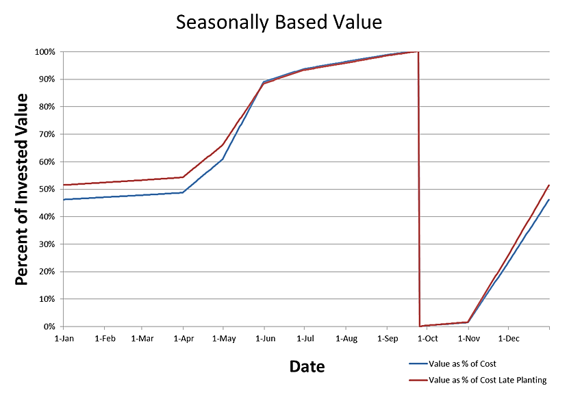
As shown in Figure, if a crop is planted late, it has a different value function. It is assumed that if the flood does not interrupt the farmer, the crops will be planted on the first plant date. Thus, late planting will only occur if the flood start plus the duration ends before the late plant date but after the first plant date. This is intended to reflect that farmers may adopt different schedules for application of watering, fertilizer, and other processes in raising the crop.

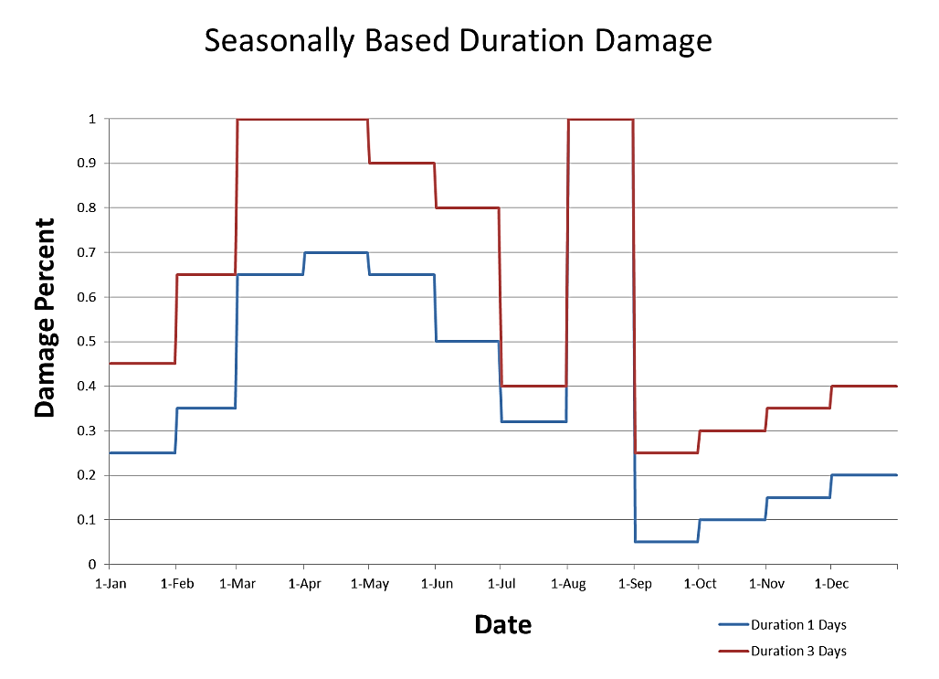
Damages also fluctuate based on seasonality. Some crops can better withstand short duration floods if they are out of critical development stages. Figure gives a general example of what seasonal duration damage relationships look like.

Generally, longer durations would yield larger losses, and more mature plants would be more robust to damage. However, as depicted in Figure, if farmers cannot harvest their crops at the proper time, the crop could be entirely lost.

Figure: Seasonal crop duration damage example.

Indirect Economic Damage

The ECAM component within LifeSim utilizes the direct damages and life loss, computed as discussed in Computational Procedure. The losses of capital and labor as a ratio of the overall available capital and labor by sector are evaluated. After labor losses and capital losses are calculated, they are submitted to the ECAM study component as inputs. ECAM then computes indirect losses.

Capital Losses

Capital loss results are computed through three steps: (i) calculating the total exposed value per county; (ii) calculating the losses per county resulting from the event; and (iii) dividing the losses per county by the total exposed value per county for all non-residential structures, which results in a capital loss ratio per county. The procedure for calculating capital loss results is listed below.

1. 1Calculate the total capital for county c (TC_c) by summing the structure and content values for all non-residential structures within county c using the following equation:
   $$TC_c = TIC_c + TCC_c + TPC_c$$

   where TIC_c is the total industrial capital for county c, TCC_c is the total commercial capital for county c, and TPC_c is the total public capital for county c.

2. 2Calculate the total lost capital by summing the damages for each structure category, as computed in the direct damages computations. The total lost capital for county c (LC_c) is calculated using the following equation:
   $$LC_c = LIC_c + LCC_c + LPC_c$$

   where LIC_c is total lost industrial capital for county c, LCC_c is total lost commercial capital for county c, and LPC_c is total lost public capital for county c.

3. 3Finally, a comparison between the lost capital for county c (LC_c) and the total capital for county c (TC_c) is expressed in terms of a capital loss ratio (CL_r). This ratio, which cannot be greater than 1 nor less than 0, is calculated using the following formula:

   $$CL_r = \frac{LC_c}{TC_c}$$

Labor Losses

To compute labor losses within LifeSim, the populations for all structures within the inventory that are impacted by the event are utilized. This means that populations in both residential and non-residential structures will be utilized to calculate labor loss based upon the population under the age of 65 at 2 PM. The justification for that assumption is that although the entire population is not part of the workforce, it is assumed that the ratio of laborers to non-laborers within the study area is fixed both geospatially and temporally. The procedure for calculating labor losses was derived from FEMA's formulas for estimating population damage (Table 13.2 of Hazus-MH 2.1 Technical Manual) (FEMA, 2020) [?]. The methodology used in LifeSim is described below.

1. 1Identify the number of people located in each impacted structure at 2 PM.
2. 2Calculate the impact duration for each structure s (I_s) in hours using the following formula:
   $$I_s = D_s + C_s + R_s$$

   where D_s is duration of flooding at structure s (hr), C_s is cleanup time at structure s (hr), and R_s is reconstruction time at structure s (hr). I_s may not exceed 8,766 hours (equivalent to one year, or 365.25 days). D_s, C_s, and R_s are defined by the user in the ECAM Data dropdown tab of the Alternative Editor dialog box.

3. 3Calculate the number of labor hours displaced for the working population at each structure (LHD_s) using the following formula:
   $$LHD_s = I_s \cdot \left(\frac{2000}{365.25 \cdot 24}\right) \cdot (P_s - L_s)$$

   where 2000 is the number of working hours per laborer per year, 365.25 is the number of days per year, 24 is the number of hours per day, P_s is the total population under 65 in structure s, and L_s is the life loss under 65 for structure s.

4. 4Calculate the total labor loss at structure s (LL_s) in hours by adding the working population labor hours displaced (LHD_s) to the working population labor hours lost due to life loss using the following formula:
   $$LL_s = LHD_s + L_s \cdot 2000$$

   where L_s is life loss at structure s and 2000 is the number of working hours per laborer per year.

5. 5Calculate the cumulative labor loss for county c using the following formula:
   $$LL_c = \sum_{s}^{n} LL_s$$

   where LL_c is the labor loss for county c in hours, LL_s is the labor loss for structure s, and n is the number of structures within county c.

6. 6Calculate total population during the day (Popday) per county using the following formula:
   $$Popday = 95\%ResidDay + 98\%WorkingCom + 80\%WorkingInd + Hotel + Visitor + 80\%SchoolEnrollmentKto12 + College + 5\%Pop$$

   where ResidDay is the daytime residential population, WorkingCom is the number of people commuting, WorkingInd is the number of people employed in the industrial sector, Hotel is the number of people staying in hotels in the census tract, Visitor is the number of regional residents who do not live in the study area, SchoolEnrollmentKto12 is the number of grade school students, College is the number of college and university students, and Pop is the census tract population.

7. 7Calculate the total available workforce for county c (WF_c) using the following formula:
   $$WF_c = \sum_{i}^{n} Popday_i \cdot (1 - EldersFrac_i)$$

   where EldersFrac is the fraction of the population over age 65.

8. 8Finally, a comparison between the labor loss for the county (LL_c) and the available labor for the county will be expressed in terms of a labor loss ratio (LL_r). This ratio, which cannot be greater than 1 nor less than 0, is calculated using the following formula:
   $$LL_r = \frac{LL_c}{2000 \cdot WF_c}$$

Indirect Economic Losses

To convert the capital loss ratio (CL_r) and labor loss ratio (LL_r) into a reduction in economic output, the ECAM system model requires information about the specific nature of the economy being analyzed. The ECAM system model determines whether the economy in question is capital or labor intensive, and what the rate of exchange is between labor and capital. Each county has a unique dataset that is used to define the specific economic characteristics assessed in the ECAM system model.

Statistics for production, employment, income, and all other economic indicators are based upon the IMPLAN (IMpact analysis for PLANning) dataset, unless otherwise indicated. Each of these datasets can distinguish up to 440 separate production activities, ten household types, and four levels of government. The dataset used for evaluating indirect economics with ECAM and LifeSim has been aggregated from the full 440 sectors to 30 sectors. Additional information on the IMPLAN dataset is available from IMPLAN Group, LLC. Additional information on the ECAM system model can be found in Lehman et al. (2013) [?].

Outputs from the indirect losses computations include the following:

• Indirect Economic Damage Report
• Indirect Employment Loss Report