LifeSim

Computational Procedure

Chapter Overview

Once all input data have been specified, the user must define the number of iterations and times of day when the hazard will occur. Note that the time of day selected is the time of hazard occurrence, not the time of warning. All computations are relative to the hazard occurrence.

The computation process is the same for each alternative in LifeSim. The program will:

1. 1Calculate agricultural damages if they are included as part of the simulation.
2. 2Prepare alternative data.
3. 3Run simulation for the user-defined number of iterations for each hazard occurrence time selected.
   1. aRedistribute the population based on first alert received and mobilization methods.
   2. bIf included, calculate life loss of exposed population.
   3. cCalculate direct economic damages if included as part of the simulation.
4. 4The average life loss over all iterations is used to determine average labor loss and capital loss for indirect economic damages.

This chapter defines a LifeSim simulation from initiation to the final state of evacuees (clear, no hazard, or low/high hazard). This chapter also discusses how the input data are prepared for each alternative and how the population is redistributed using evacuation groups and vertical evacuation. Agricultural damage, property damage, and ECAM are based on maximum conditions and/or duration.

Preprocessing - Preparation of Alternative Data

Preprocessing the Hydraulic Data

Before the warning and evacuation simulation can begin, the hydraulic data are processed to define a flood time-series at each structure and road segment. This process extracts the necessary data from the hydraulic input during the simulation process. When time-dependent hydraulic data are used as input (all options except Summary Grids), depth and velocity hydrographs are extracted from the hydraulic data at each structure and road. All other necessary hydraulic parameters can be derived from those data such as arrival time, instantaneous depth times velocity, or duration of flooding. The preprocessed hydraulic data are saved with the model and can be used for multiple simulations as long as there are no changes to the road network, structure inventory, or hydraulic input.

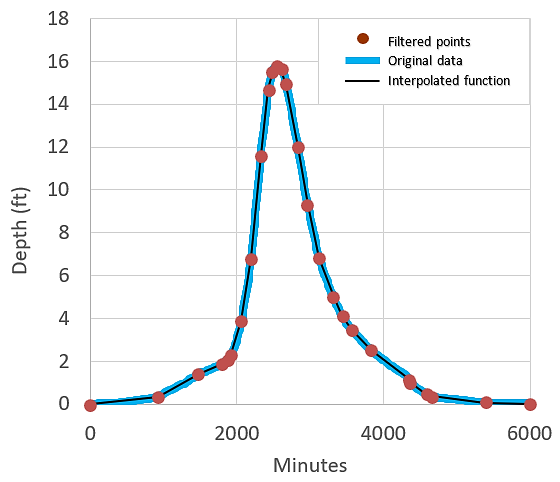
In order to conserve computational time and memory, the depth and velocity hydrographs are simplified to reduce the number of data points. The Ramer-Douglas-Peucker algorithm is used to reduce the hydrograph points as demonstrated in Figure. The algorithm concentrates data points in regions of the hydrograph with sharp changes and thins the data points where change is minimal between points and a linear interpolation can represent the curve. LifeSim uses a default tolerance of 0.01 for eliminating points. In Figure, the original hydraulic data contained 6,000 data points (blue line) but was reduced to 27 points (orange) using the Ramer-Douglas-Peucker algorithm. LifeSim applies a linear interpolation between the remaining data points with very little error introduced (black line). The strategy is particularly useful for reducing memory during long dry periods where zero depth data storage is not needed. Fewer data points also significantly reduce simulation lookup times when comparing hydraulic data to the willingness to enter a flooded road, for example.

Figure: Example of Ramer-Douglas-Peucker hydrograph simplification.

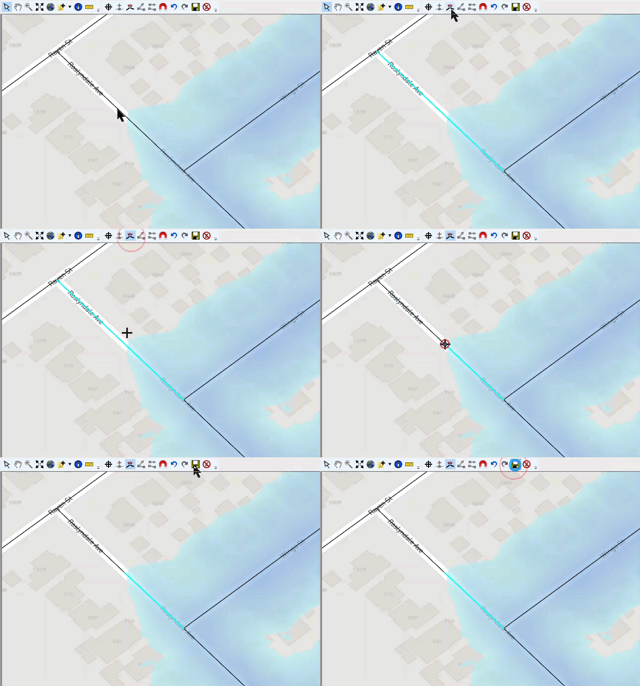
In structures, the depth is sampled from the terrain at the structure point. For roads, the midpoint of the road is used as the sampling point and the depth is then reduced by any vertical offset. The midpoint assumption may result in problems for particularly long or steep roads (see Linework). Conditions may change along the length of road that should be represented with more detail. In this case, users should divide the road into multiple representative segments. As demonstrated in Figure, the Roslyndale Ave single road segment is now sampled at two locations: once at the midpoint of the dry segment and once at the midpoint of the flooded segment.

Figure: Example of dividing LifeSim road segment to better sample hydraulic conditions at midpoint.

Preprocessing the Road Network

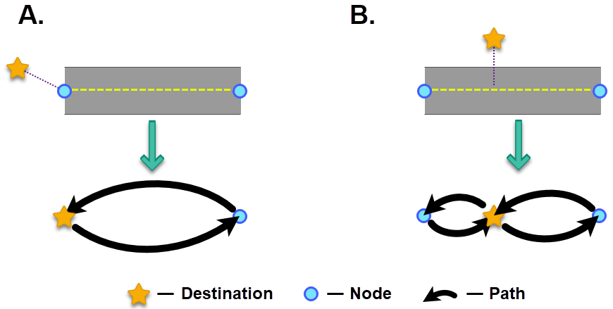
The road network is imported as GIS linework (a series of polyline segments for roads and points for destinations) and pre-processed for simulation. LifeSim first assigns each node in the network a node identification (ID) value. Then, LifeSim identifies road segments as either one-way or two-way. If the road is identified as two-way, the road is split into two components: one segment in one direction and another in the reverse direction, as shown in Figure.

Figure: Preprocessing of the road linework.

On the other hand, if the road is identified as one-way, only a single segment and direction are needed. Segments are connected based on their coincident start point or endpoint locations in GIS. Each line segment has several properties besides the starting and ending nodes including length, unimpaired travel time (at free-flow speed), and other attributes used to determine the fastest path to a destination.

Destinations are related to the road network by road segments with the shortest perpendicular distance to the destination points. If a destination is located nearest to a line segment's endpoint (side A in Figure), then LifeSim identifies that node as a destination. If instead a destination is between the start and endpoint of a segment, then the segment is split so that traffic can approach the destination from both sides. A new node is inserted where the line was broken and it becomes the destination node (side B in Figure).

Figure: Setting a destination point. Panel A: If the closest line to a destination point is at an end point, then the end node is set as the destination. Panel B: If the closest line to a destination point is between start and end nodes, the line is split at the nearest point and the new node is set as the destination.

Now that all the road and destination connections are represented, LifeSim will find the fastest path from any node along the road network to a destination. The optimal path (a.k.a. shortest travel time) to a destination is found using Dijkstra's shortest path algorithm with a binary heap data structure to improve efficiency. From each node, the next node on the fastest path to a destination is stored, resulting in a table similar to Figure. Although several pathfinding mechanisms are available (A*, D*, and others), Dijkstra's method was selected for its ability to quickly determine shortest paths for all nodes in the network.

The lookup table is used to determine the fastest route to a destination from any node in the network. For example, the shortest path from node #5 in Figure is 5, 4, 2, 1, 0, destination. In LifeSim, the user may select to limit the destinations an evacuee will initially consider. For example, evacuation orders may dictate to stay away from a certain area. To accommodate the categorization, a unique table is constructed for each EPZ (where destination assignments are made). The full network graph includes all allowable destinations with the fastest path to a destination defined for each node.

Figure: Example road network and fastest pathway lookup table.

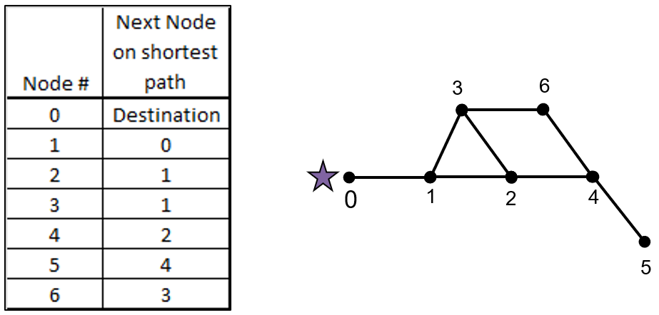
During the simulation, the starting road network is updated with traffic density and flood information. Vehicles traveling the road network may encounter traffic or flooding, in which case they would potentially re-route their course (more details in Evacuating with Traffic Simulation). For example, if a traffic jam is on the segment from node 2 to 1, a re-route may select a diversion through node 3 as the fastest way to reach the destination.

Preprocessing the Structure Inventory

The structure inventory includes attributes assigned to each structure. Before an evacuation iteration starts, the structure inventory must be updated with additional information such as:

• Structure stability criteria based on the user-defined rules.
• Which EPZ the structure is in.
• Which output polygon the structure is in (for summarizing results).
• Initial evacuation path from the structure to a destination.

Each structure in the inventory is geographically associated to its assigned EPZ polygon, output summary polygon, and closest road segment. The EPZ assignment allows each structure to be associated with an initial road network graph. Once the closest road to a structure is identified, the initial path for evacuation can be defined. Each of the two nodes on the nearest road segment has a defined path to the nearest destination. The faster of the two directions is selected based on the travel time to those nodes from the entry location on the road, plus the time from that node to the destination.

Preprocessing for Each Iteration

Each iteration is a complete simulation of the warning, evacuation, and subsequent consequences for a single event. After each iteration a sampling of all the uncertain parameters occurs. This sampling happens at the beginning of each new iteration. The information in Preprocessing - Preparation of Alternative Data above is defined once for each alternative because it does not change with each new iteration. This is the outermost loop of LifeSim's Monte Carlo simulation, as shown graphically in Figure.

The random sampling process begins with preparing iteration seed numbers for use in a random number generator. The reason for seeding the random number generator is to make results reproducible with the same input. Otherwise two users with identical input could have different results. Each iteration is given a seed number that is quasi-random, unique, and reproducible. For example, if the alternative specifies 100 iterations, the model will create 100 quasi-random seed numbers in a seed set.

Figure: Nested loops used in Monte Carlo simulation.

Each alternative may be repeated for different times of hazard occurrence with the same number of iterations each. The same seed set is used for each time of day so that the i-th iteration for one time of day has the same seed as all i-th iterations for other times of day. This allows users to compare results more directly between times of day (all else being equal) and produces a discernable pattern in the results. Note the middle two loops of Figure.

Within each iteration, a random number generator is defined for sampling uncertainty and seeded with the iteration's random seed number. Then the warning, evacuation, and consequences simulation proceeds to its end and the next iteration begins.

The Monte Carlo simulation allows users to see the impact of uncertain parameters on the range of model results. Confidence in the results is built as several iterations with different parameters show agreement. More discussion of the uncertainty sampling is included in Uncertainty and Sampling Methods with an exhaustive list of parameters sampled during each iteration.

Note that this process is not testing for convergence on some parameter, but merely a user-defined number of iterations which provides output as a distribution of results. The number of iterations specified is important. It is up to the user to determine if enough iterations are computed to reach convergence of results. The user must balance the increased run time from each additional iteration with the accuracy and confidence gained in the results.

Warning Function Sampling

The warning notification and timing functions are unique for each EPZ. With each iteration, different values for the warning delays are sampled (imminent hazard identification, hazard communication delay, warning issuance delay, first alert diffusion delay, PAI delay). The sampled imminent hazard identification, hazard communication delay, and warning issuance delay have one value per EPZ defining the time it takes from discovery of a hazard to when an evacuation warning is first released to the public. The below equation is used to calculate when warning is first issued for each EPZ.

$$WI_{EPZ} = HO + IH_{EPZ} + CD_{EPZ} + ID_{EPZ}$$

where:

WI_EPZ = Warning Issuance Time at specified EPZ.
HO = Hazard Occurrence Time.
IH_EPZ = Imminent Hazard Identification Time for specified EPZ.
CD_EPZ = Communication Delay of imminent hazard to EPZ personnel.
ID_EPZ = Issuance Delay of warning to the public at specified EPZ.

The first alert diffusion delay and PAI delay data are sampled using curve sampling techniques to produce population delay functions for each EPZ. The sampled first alert and PAI functions refer to a percentage of the population warned (or mobilized) over time. Since LifeSim is an agent-based model, the population characteristics must be distributed down to the agent level as described in Evacuating Groups and Their Attributes.

Population in Structures

The population represented within a LifeSim structure inventory is dynamic, representing typical movement of people throughout the day and night such as attending school or frequenting a business and returning home in the evening. The structure inventory has populations defined for daytime and nighttime that consider these diurnal shifts. However, LifeSim needs to track the population at any time because the exact time of a flood hazard and warning can have uncertainty. LifeSim does this by defining periods of daytime, nighttime, and transitional periods.

During the transitional periods, the population is interpolated between the imported daytime and nighttime populations. Transitional periods are from 4 AM to 10 AM and 5 PM to midnight. Examples in Figure and Figure are for two different types of structures with a representative population of 100. In a typical residential structure (Figure), the population is higher at night and lower during the day with transitions during the morning and late afternoon. By contrast, a typical commercial or public building might have a higher daytime population and lower nighttime population (Figure).

Figure: Population interpolation example: typical residential structure.

Figure: Population interpolation example: typical commercial/public structure.

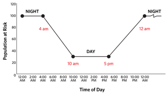
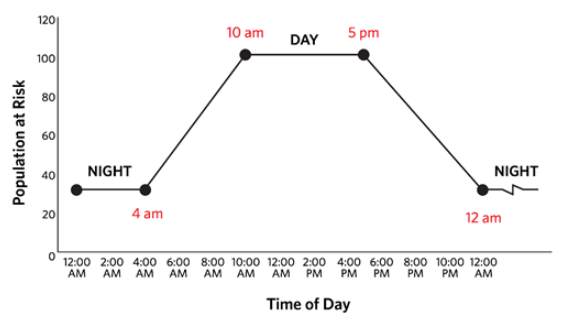
It is most appropriate to select the population based on when the warning is first released to the public because that is when people begin to react to the flood. Initial population distribution is interpolated at each structure using the sampled warning issuance time for each EPZ. For example, if the hazard occurrence is set to occur at 2 AM and the warning is issued 8 hours prior to the hazard occurrence at 6 PM, then LifeSim will use the interpolated population at 6 PM. Since each EPZ's warning issuance time can be unique, they may all use different population snapshot times.

Each EPZ uses its own warning issuance time to define the population. However, population shifts between EPZs are not tracked in LifeSim. For example: if someone has evacuated from one EPZ and travels to another (i.e., a person gets a warning at work in one EPZ but lives in another EPZ that is not warned until later). Also, the diffusion of the first alert may take several hours. In which case, people who have not been warned may continue with their day as normal and change locations. These people are included at their first location and not tracked to a new location having different warning and evacuation parameters. Likewise, there is no accounting for commute time. Everyone must be inside a structure to start the simulation.

Four factors that define the warning issuance time in LifeSim are:

1. 1Time of the hazard occurrence
2. 2Imminent hazard identification time
3. 3Hazard communication delay
4. 4Warning issuance delay

Evacuating Groups and Their Attributes

With the starting population known, it can be broken up into evacuating groups. An evacuating group travels together regardless of mode of transportation (vehicle or pedestrian). The user specifies the number of people in each evacuating group by occupancy type (see Evacuating Group Size). Groups are partitioned from among the building's population by group size with any remainder comprising the last group. Evacuating groups may be less than the group size, but not larger.

An evacuating group stores information such as:

• The number of individuals in the group.
• The structure they started in.
• Availability of roof/attic access.
• Time of first alert.
• Time of mobilization (PAI, if applicable).
• Evacuation mode: in a vehicle or on foot.
• If in a vehicle, vehicle type (high or low clearance).
• Sampled stability function for defined mode of transportation.
• Depth of flooding they are willing to enter (fording depth).
• If reaching a traffic jam, whether or not they will turn around.
• The evacuation route they are on.
• Where they are on the evacuation route.
• Current speed on the evacuation route.
• Memory of flooded roads encountered during evacuation.
• If they reach their destination.
• If they get caught while evacuating.

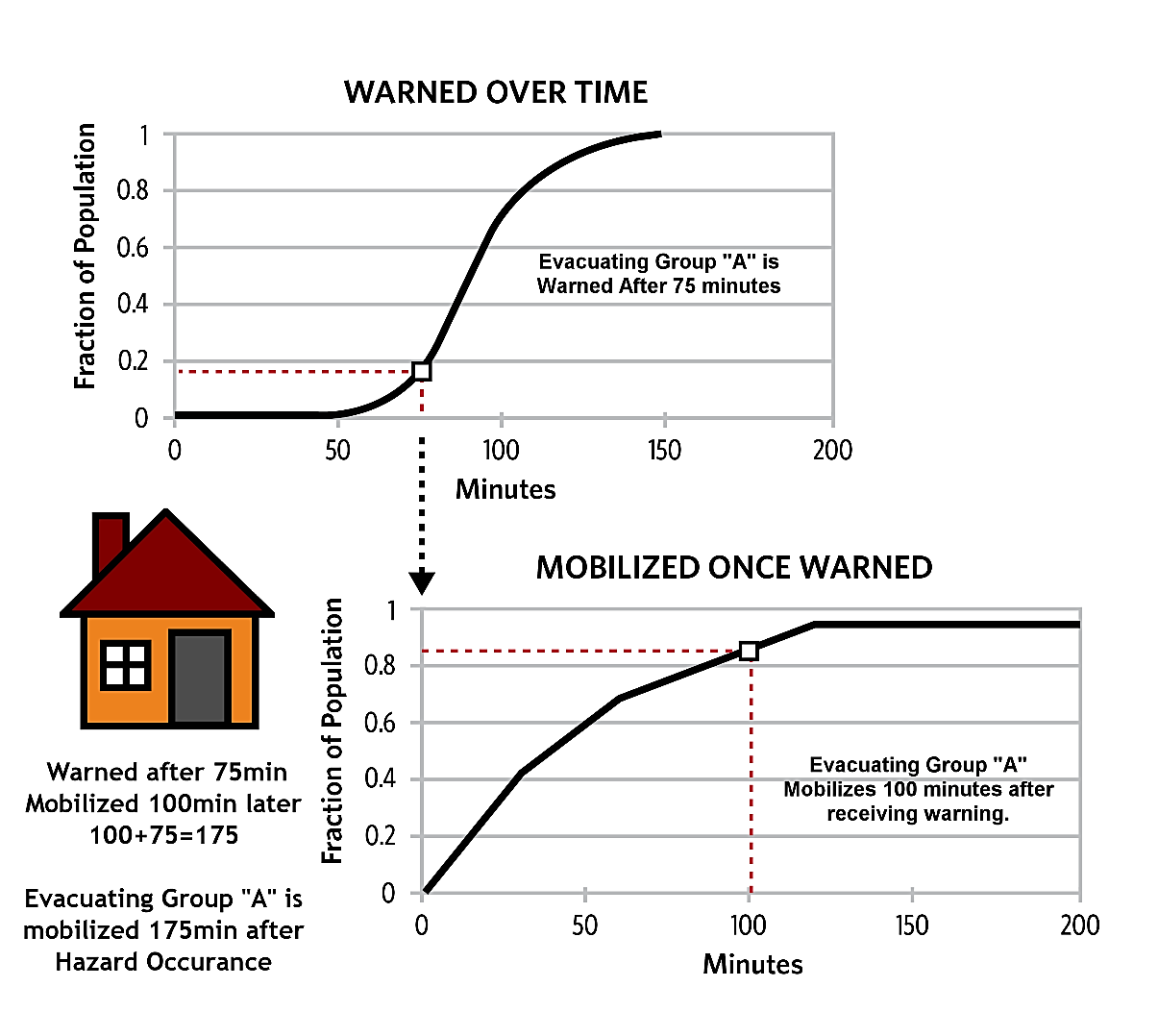
Each evacuating group samples from the first alert and PAI delay functions for that group's emergency planning zone to determine when the group receives a warning and when they take protective action. Using the sampled first alert and PAI functions for each EPZ along with the evacuation parameters defined at the occupancy type (Evacuation Parameters Defined by Structure Occupancy Type), every group is randomly assigned a time of first alert and time of PAI (Figure). The functions represent a fraction of population over time. By sampling with many structures and evacuating groups over the whole EPZ, the sampled population warned (or mobilized) over time approximates the first alert diffusion function (or PAI function). These parameters may be sampled per evacuating group or per structure depending on whether they are warned and mobilized together.

Figure: Example of how the first alert and PAI functions are sampled to get time warned and time mobilized for each evacuating group in LifeSim.

Attributes Assigned to Individuals

Most operations during the evacuation simulation are done at the evacuating group level, but individuals show independence in LifeSim especially during vertical evacuation and when calculating their survival in hazardous conditions.

An individual is defined by their:

• Mobility (limited or able-bodied)
• Highest position attained in a flooded structure (roof, attic, or top floor)
• Ability to swim

Each person within the population has either limited mobility or is able-bodied and can swim or cannot. Based on their mobility, they have a chance of reaching higher levels than the top floor of the structure during vertical evacuation.

Parameter Sampling for Structures

A number of parameters are re-sampled for each iteration and assigned to individual structures. Two general categories of parameters are sampled: those related to consequence calculations and those related to warning and evacuation.

The sampled consequence related parameters include:

• Foundation height
• Depth-damage function
• Property values (including structure, contents, vehicles, and other)
• Structure submergence criteria
• Structure stability function

All of the listed parameters are defined by occupancy type except structure stability. Structure stability criteria are sampled per structure. If two structures have the same stability criteria assigned, they could have different sampled stability thresholds depending on if uncertainty was defined. The stability is sampled per structure to account for the natural variability in materials and construction practices, even within the same housing tract.

The height of each story and attic is imported with the inventory (no uncertainty), but the foundation height may have uncertainty that is sampled and assigned to the structure. Uncertainty about foundation heights is defined at the occupancy type level. Each structure has a foundation height attribute. The structure's occupancy type uses the uncertainty defined at the occupancy type level with the static value at the structure to sample a new foundation height for the structure. Property values use the same approach as foundation height to sample uncertainty. Depth-damage functions are sampled once per occupancy type and use curve sampling to compute new depth-damage functions for each iteration. Submergence criteria are sampled once per occupancy type for each iteration.

Evacuating the Structure

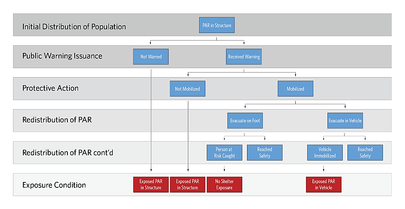
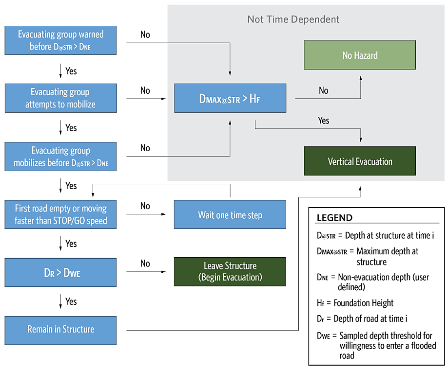
All of the preprocessing of data is necessary for the evacuation simulation to begin. Now that the warning and mobilization times are known for each evacuating group, the decision thresholds are known for each evacuating group, and the time series of depths and velocities are assigned to each road and structure, comparisons can be made between these values to decide if the group tries to evacuate or not. The people at risk could get exposed to hazardous conditions either in a vehicle, in a structure, or have no shelter, as shown in Figure.

Figure: LifeSim computation process pre-exposure.

Before evacuees can mobilize, the conditions outside the structure must be relatively safe to allow evacuation. The program does the following checks:

1. 1Current depth at structure. Is depth above or below the non-evacuation depth?
2. 2Look at road nearest structure. Is depth on road above the willingness to enter depth?
3. 3Number of vehicles on road. If nearest road has reached vehicle capacity based on effective vehicle length and road length, the evacuating group will wait until next time step.

Some people may decide not to mobilize at all if the evacuating group is part of the sampled fraction on the PAI function above the maximum mobilization rate, regardless of the depths and traffic. People who do not evacuate from the structure will be able to vertically evacuate within the structure if needed. The full logic tree is shown in Figure.

Figure: Decision tree for beginning to evacuate or remain in structure, with traffic simulation.

Evacuating Without Traffic Simulation

LifeSim gives users the ability to estimate the number of people who leave a flooded area without actually modeling the evacuation process. This is done by comparison of the depth at the structure and the non-evacuation depth. If the evacuating group attempts to mobilize before the depth at the structure exceeds the non-evacuation depth, they are assumed to succeed in their evacuation and are removed from the exposed population. Turning off the traffic simulation also includes walking evacuation since pedestrians use the road network.

The benefit of this option is much faster computation times because the road network is not a part of the simulation and no vehicles are tracked. The downside is no consideration of people caught while evacuating and therefore no life loss on roads. It is best to use this function when there is expected to be plenty of time to evacuate everyone who can and chooses to evacuate or when the conditions dictate this option. Examples of this may be long, narrow canyons with short warning times where walking up the hillside is the fastest way to safety or urban settings where most people do not have vehicles.

Evacuating With Traffic Simulation

Once an evacuating group leaves their structure, they enter a dynamic (time-dependent) environment where they interact with the road network, other vehicles, and flood water. Each evacuating group (whether in a vehicle or on foot) is tracked as they travel from their structure along the road network to a destination. The conditions and position of evacuating groups are updated during each evacuation time step, representing the bulk of LifeSim calculation time. If groups reach a destination, they are considered cleared and removed from the simulation. If they contact flood water, the vehicle and human stability functions determine if stability is lost or not. Figure presents an overview of the vehicular evacuation logic; more detailed descriptions follow.

Figure: Overview of vehicular evacuation logic and how vehicles are assigned to a hazard zone.

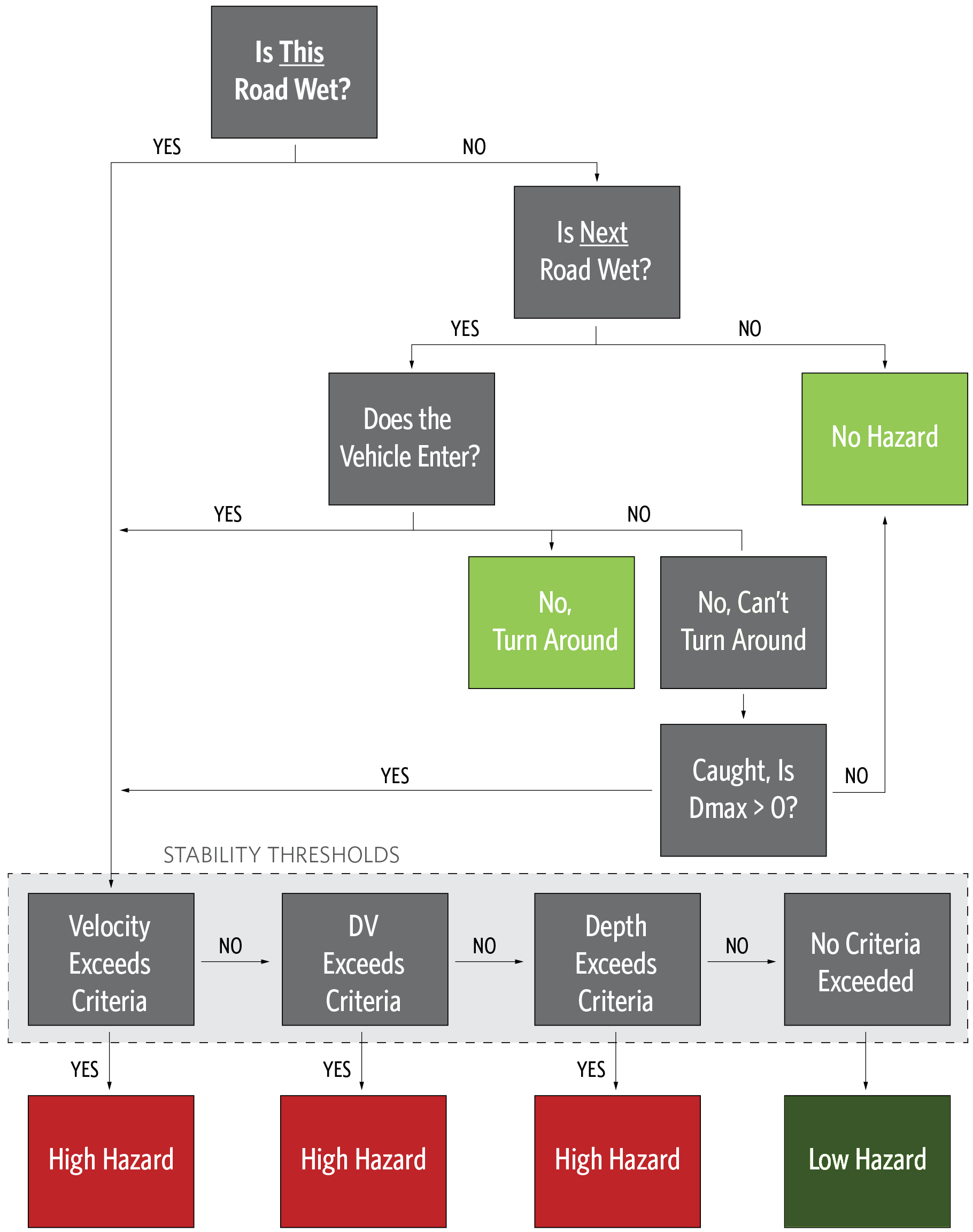
Vehicle movement is predicted using vehicle speed and the allowable time to predict the distance they can travel. If the traveled distance is farther than the distance to the end of the road segment, the vehicle reaches the end of that segment and has a chance to enter the next segment. At this point, the vehicle must decide whether to continue driving on the new segment. Assuming the next road segment is dry, the vehicle continues with an updated speed based on the next segment's CFCC attribute (or at stop-and-go speed if wet). The distance traveled over the remaining time in the time step is calculated and the process repeats on each segment traveled until the full time step is used.

Vehicles travel the road network to their intended destination at the free-flow speed unless they are impacted by something to slow them down or they decide to re-route. A vehicle may also become "caught," in which case it stops moving and remains in its current location.

The conditions that may divert, catch, or slow a vehicle are:

1. 1Traffic congestion: (see Evacuation Parameters Defined by Alternative for more information on setting evacuation parameters).
   1. aAs traffic density on a road increases, vehicle speed decreases according to Greenshields' two stage formula (Equation and Equation) until it reaches the minimum "stop-and-go speed," resulting in a traffic jam (traffic jam = vehicles ahead moving at stop-and-go speed). The traffic density is calculated once per time step and includes all the vehicles on the road between a vehicle's starting position and the look-ahead distance. Each road segment is broken into sub-segment bins where the number of vehicles is tracked. Bin lengths are not adjustable but calculated to reduce long roads into realistic road lengths where cars can be considered to impact each other's speeds. Before density is calculated, newly mobilized vehicles are added to the road. If a vehicle enters a new road segment with a different free-flow speed in the same time step, the same proportional reduction in speed is used for that segment also (there is only one calculation of density per vehicle per time step).
   2. bIf confronted with a traffic jam, some vehicles will attempt to find a faster alternate route. As noted above, the density is only calculated at the beginning of a time step so the decision to re-route for traffic can only be made at that time.
   3. cIf the spillback function is turned on, an additional correction may be applied to the vehicle location. The effective vehicle length is used to make sure the number of vehicles on a road segment is physically possible given the number of lanes, length of the road segment, and space taken by the average vehicle. If too many vehicles are on a road segment at the end of the time step, the spillback function pushes the last vehicle to enter back onto the previous road segment. This continues until each road segment is at or below its physical capacity.
2. 2Flood water: any water covering the road with depth greater than the vertical offset height.
   1. aA vehicle may decide not to enter a flooded road segment if the depth is greater than its fording depth (seeWillingness to Enter Flooded Roads for more information). In that case, it will attempt to re-route. The decision point to re-route for flooding is at the start of each road segment and could happen multiple times in a single time step.
   2. bIf the vehicle tries to re-route for flooding when on a one-way road, it is caught, but may remain dry and safe. For example, if a vehicle tries to enter a flooded freeway from a dry on-ramp, they may get caught on the on-ramp but never actually get wet.
   3. cIf a vehicle re-routes for flooding and is able to turn around, flood water may block all possible paths (all deeper than the sampled fording depth). If there are no valid routes, then the vehicle will be caught.
   4. dA vehicle may be caught if it loses stability on a flooded road. This can happen when flood conditions change rapidly on the road or when a vehicle is willing to enter a road it cannot safely navigate.
   5. eWhen driving through water, all vehicles move at the stop-and-go speed for that road segment.
3. 3A vehicle caught in water: If a vehicle is confronted with another vehicle caught on the road ahead and the road is wet, it will attempt to re-route. If the vehicle in front is caught and the road is dry, the confronted vehicle will make its own decision to enter or re-route, per (2) flood water. This case assumes if the evacuating group sees a stalled vehicle in water, they will consider it unsafe and not attempt to cross.

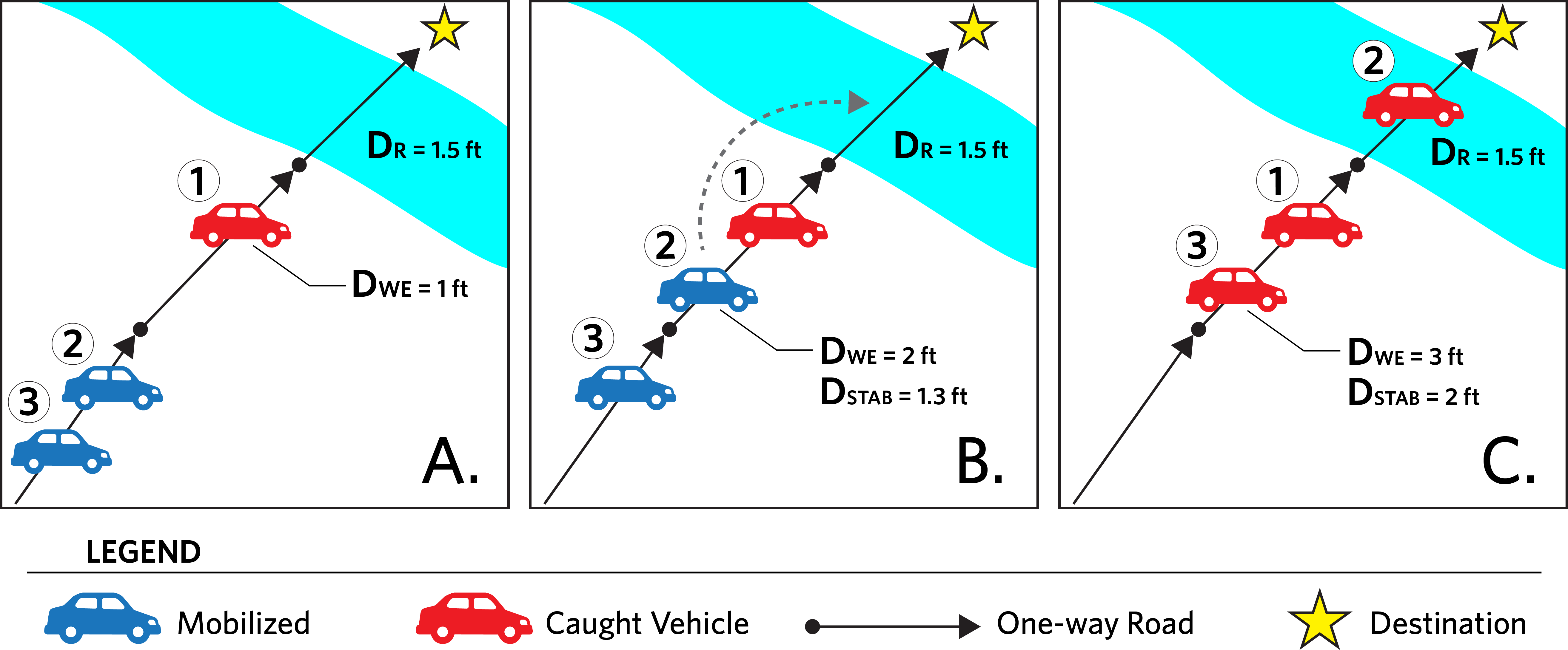
Examples of vehicles in conditions from (2) flood water and (3) a vehicle caught in water are discussed in reference to Figure.

• Panel A: Vehicle 1 approaches a flooded road and decides not to enter because the depth is higher than its willingness to enter depth (D_R > D_WE). Vehicle 1 is caught at that location because it cannot turn around on the one-way road.
• Panel B: a second vehicle approaches Vehicle 1. Since the road in front of Vehicle 1 is clear of vehicles and Vehicle 2 has a willingness to enter the flooded road (D_WE > D_R), Vehicle 2 passes Vehicle 1 and enters the flooded road. Unfortunately, Vehicle 2 has a low vehicle stability threshold and loses stability on the flooded road (D_STAB < D_R, recognizing that the stability function also includes velocity considerations).
• Panel C: a third vehicle approaches, also willing to enter (D_WE > D_R) and with stability criteria high enough to navigate the flooded road successfully (D_STAB > D_R). However, the road is "blocked" by caught Vehicle 2, so Vehicle 3 does not enter the flooded road and is caught in line behind Vehicle 1. Vehicle 1 and 3 represent the beginning of a traffic backup on this road, assuming the spillback function is turned on.

Figure: Examples of decisions to enter a flooded road. Panel A shows a vehicle (1) that will not evacuate across the flooded road. Panel B shows a vehicle (2) that is willing to enter and loses stability while trying to cross the flooded road. Panel C shows a vehicle (3) that is not willing to try and cross the flooded road with a stalled vehicle (2) on it.

Re-routing Vehicles

Re-routing for traffic and re-routing for flooding are slightly different processes. Not all vehicles will attempt to re-route for a traffic jam (condition [1b] traffic congestion, traffic jam), but all vehicles will attempt to re-route for the other flood-caused conditions ([2] flood water and [3] a vehicle caught in water). During preprocessing for the iteration, each vehicle samples whether it will attempt re-routing due to a traffic jam, governed by the "fraction who re-route in a jam" parameter.

Vehicles trying to re-route will attempt to find a new fastest path to a destination regardless of their initial EPZ destination assignment constraints (all destinations are allowed). If a faster path to a destination is available, it will be selected.

Vehicles are allowed to make a U-turn on most two-way roads. However, limited access highways (CFCC code A10-A29) and one-way roads do not allow U-turns, and vehicles will have to go to the end of the road segment before turning around.

Vehicles trying to re-route for traffic reasons have near real-time knowledge of the traffic conditions on the whole road network. The road network graph is continuously updated with current traffic conditions during the evacuation simulation, based on the "live traffic update interval." Basically, this assumes that people will consult a device such as a smartphone with up-to-date traffic information when re-routing due to traffic conditions.

Each re-routing vehicle also retains knowledge of every flooded road that caused it to re-route and will not attempt to use that road segment again. Flooded roads that were successfully crossed may be reused as part of an alternate path. Flooded roads blocked by a caught car are not known to the vehicle unless already encountered.

It is assumed that each vehicle re-routing due to flooding does not use live traffic and uses the initial road network graph updated from each agent's flooded road memory to find their fastest path to a destination.

Evacuating on Foot

Evacuating on foot is similar to vehicle evacuation but has some key differences and simplifications. Pedestrians evacuate in groups that stay together just like a vehicle. They also use the same road network as the vehicles but are handled independently of the traffic even when they are on the same road. Key differences for pedestrians are:

• There is no pedestrian spillback function or pedestrian density considerations. Roads are expected to handle the full pedestrian population.
• Pedestrians always move at the pedestrian evacuation speed; there is no change in speed for "pedestrian traffic jams."
• Pedestrians do not re-route for traffic (vehicle or pedestrian).
• All pedestrian groups are willing to enter a flooded road with less than two feet of water and try to re-route if confronted by deeper water.
• To get caught, the human stability function is considered for the group as a whole while on flooded roads.

The default setting in LifeSim 2.0 is for full vehicular evacuation because pedestrians are typically a small fraction of the evacuating population. Two exceptions to this default assumption may be long, narrow canyons with short warning times where walking up the hillside is the fastest way to safety or urban settings where most people do not have vehicles.

Caught while Evacuating

Being caught while evacuating is not the same as losing stability. A caught vehicle may be on dry land with nowhere to go (see Vehicles 1 and 3 in Figure). Once an evacuating group is caught, they are subjected to stability criteria that may or may not be exceeded. All members of the evacuating group are placed in the high hazard or low hazard zone together.

For vehicles, first the vehicle stability is checked against the maximum conditions of the road segment where they were caught. If surpassed, the human stability criteria are also checked. This assumes that under certain conditions, a person may exit their car and walk/swim to safety. If vehicular stability is exceeded but human stability is not exceeded, the group will be in a low hazard zone. If both human and vehicle criteria are surpassed, the evacuating group is placed in the high hazard zone. If no stability criteria are surpassed but the vehicle was on a wet road, they are placed in a low hazard zone.

For pedestrians, only the human stability function is considered (including the portion with swimming ability, if applicable).

Everyone who is not caught either reaches a destination and is safe and cleared, or remains in their structure and is subject to the vertical evacuation criteria.

Vertical Evacuation Within Structures

A subset of the population remains in their structure either by choice or because water arrived before they could mobilize. These people are subject to the structure stability and submergence criteria. In LifeSim, all people will move to the highest story of a building, and some will continue to move up into an attic or onto the roof as their sampled mobility and access allows. Figure demonstrates the vertical evacuation logic.

Figure: Vertical evacuation logic in LifeSim assuming the structure remains stable.

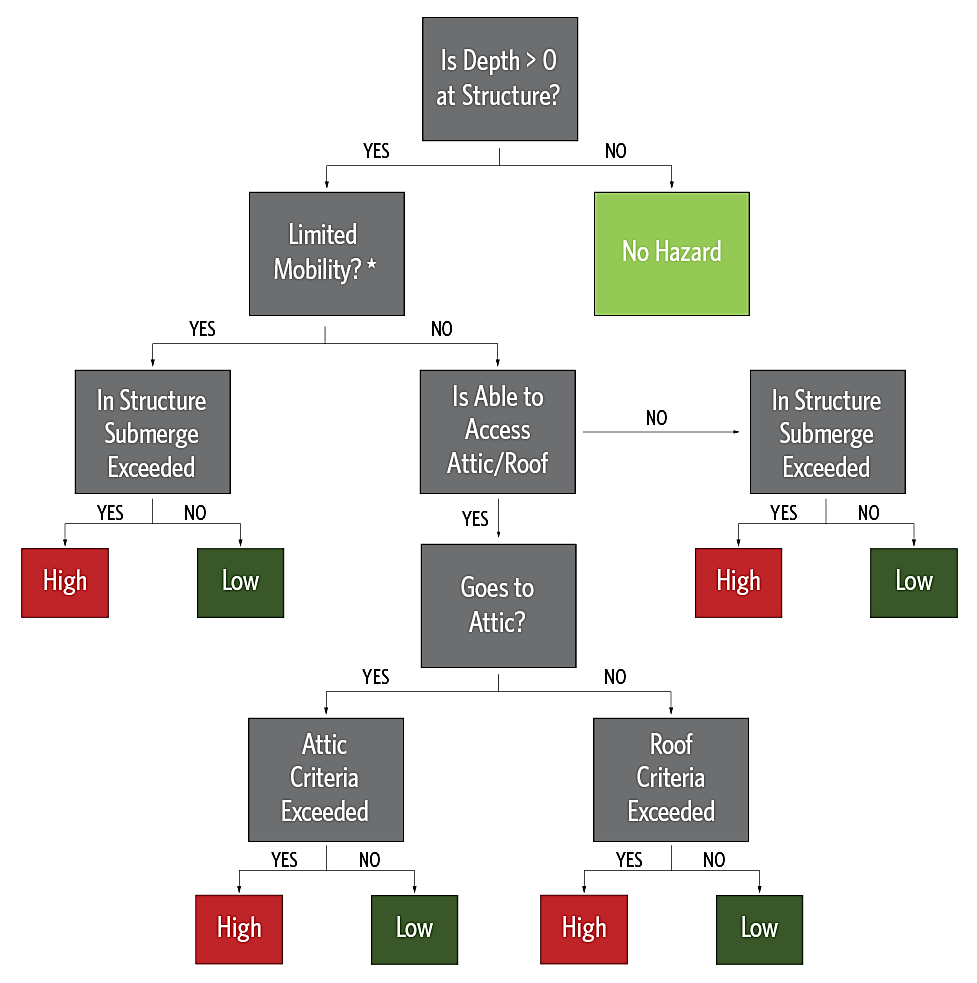
Vertical evacuation is not time-dependent. The logic employed by LifeSim assumes that people will continue to move vertically within their structure as fast and as high as possible to stay above the rising water. The rate of water rise is not considered – only the maximum conditions. However, vertical evacuation is not possible if the maximum conditions would lead to collapse of the structure (by comparison to the sampled structure stability function). In that case, all occupants are automatically placed in the high hazard zone and the structure and contents are considered a total loss.

The vertical evacuation calculation begins with subtracting the sampled foundation height from the maximum depth at the structure. If the resulting in-structure depth is less than zero, the occupants are still considered low hazard to account for people who could become trapped in a basement or those who leave the structure (not intending to evacuate) and are impacted by the flood waters outside their house. Although rare, several stories of this risky behavior were documented in the research to develop the fatality rate functions. If the maximum depth at a structure is less than or equal to zero, then there is no hazard, no further calculations are required, and all occupants are deemed safe.

If the interior depth is above zero, the next calculation is for the stability of the structure. Each structure has a sampled stability function (discussed in Preprocessing - Preparation of Alternative Data and Preprocessing for Each Iteration). The structure stability criteria are tested against the time series of depths and velocities at the structure to determine whether the structure collapses at any point during the simulation. This process only determines total collapse of a structure. Case histories have identified instances of partial collapse where water may remove a wall and reduce the protection provided by the shelter. If the stability function is exceeded, all people are placed in the high hazard zone and no vertical evacuation is computed.

Once it is established that the structure is flooded and does not collapse, LifeSim must determine how high each occupant is able to move within the structure. People with limited mobility are assumed to move to the highest floor but no higher. This simplification neglects the impact of co-occupants to assist those with limited mobility (elderly, infants, disabled) and represents the most common condition. Several stories of survivors and fatalities in structure flooding were consulted (Development of Flood Fatality Database). The high hazard fatality rate function includes several cases of those with limited mobility assisted by others. Regardless of their actual position in the structure, their limited mobility in a flooded structure seems to constitute a high hazard situation.

Those without limited mobility have the possibility of moving into the attic or roof. For each person in each group, the roof/attic access (Probability of Access to Roof or Attic) is sampled to determine further vertical movement then split between those who go to the attic or the roof (Fraction to Roof vs Attic) to determine final location.

Once everyone's final position is known, the structure submergence criteria are applied (as discussed in Submergence Criteria). The submergence criteria represent the threshold depth between high and low hazard zones. If the interior depth exceeds the threshold, the occupant is placed in the high hazard zone, and all others are in the low hazard zone.

A special case exists for structures with zero stories. This represents a place where people are gathered outdoors – perhaps a park, campground, or agriculture field. In this case, the structures around the people provide little protection and they are subjected to human stability criteria as if they are pedestrians caught at their structure.

General Modeling Guidelines

The user should consider the following when running a simulation:

• The decision to enter a flooded road for evacuating groups is a function of depth. A person's inability to accurately estimate depth while in a vehicle or on foot is not taken into account.

• Although the model currently does not have convergence options for determining the number of iterations, convergence testing can still be calculated in post-process. Results by iteration are available in table form which can be exported or copied for use in other applications. Convergence testing can then be performed on the desired result (e.g., total life loss, total damage) by iteration.

• A partial evacuation is possible by deactivating all destinations for an EPZ; no one will leave their structures. Another option to simulate partial evacuation by EPZ is to set the maximum % initiated to zero in the PAI function. In this case, everyone will remain in structures and vertically evacuate (a.k.a. sheltering-in-place) and will be subject to the maximum flood conditions at that structure.

• For evacuating vehicles, the evacuation time step and look-ahead distance are critical to ensuring vehicles do not skip over a traffic jam. As evacuation time step is increased, vehicles can travel farther in a single time step. If the look-ahead distance is too short, vehicles may have initial speeds that do not reflect a traffic jam that they will reach in a single time step.

• By manipulating the EPZ's simulate traffic parameter (Emergency Planning Zone), the user can turn off simulating traffic by EPZ. The traffic simulation process can be very intensive and take a long time. It is common practice to turn off traffic simulation if the hazard arrival time is long enough for people to reach safety for those that will take protective action in areas that will be impacted.