Internal Erosion Suite

First-Order, Second-Moment Reliability

The Taylor series is a method to estimate the expected value (mean) and standard deviation of a limit state, given the means and standard deviations of the parameters. This method is termed a first-order, second-moment (FOSM) method, as only first-order (linear) terms of the series are retained and only the first two moments (mean and the standard deviation) are considered. The Taylor series method of reliability analysis has been used by USACE for many years to compute the reliability index and probability of unsatisfactory performance.

Only the first two moments (mean and variance) represent the probability density function in the reliability analysis, and all higher order terms are neglected in the Taylor series expansion used to estimate the mean and variance of the natural logarithm of the factor of safety. When using the reliability index method, no knowledge is needed of the exact probability density function that represents random variable.

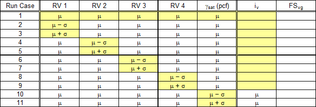
Figure shows the seepage analysis run cases for a single headwater level of interest after estimating the mean and standard deviation of each random variable (RV). The first run case uses the mean (μ) of all random variables to obtain the mean value of the vertical seepage exit gradient (i_v). In subsequent run cases, each random variable is adjusted up or down by its standard deviation (σ) while using the mean values of all other random variables. The vertical seepage exit gradient is from seepage analysis for the various permutations. Run Cases 10 and 11 involve the saturated unit weight of the landside blanket, which is used to calculate the critical vertical seepage exit gradient for heave/blowout. Since no changes to the seepage model are required for these two run cases, the mean vertical seepage exit gradient from Run Case 1 is used. After obtaining the vertical seepage exit gradient for Run Cases 1 to 9, the factor of safety against heave/blowout (based on vertical seepage gradients) is calculated for all eleven run cases.

Figure: Seepage analysis run cases for first-order, second-moment reliability analysis.

The mean and standard deviation of the natural logarithm of the factor of safety are obtained using the mean, standard deviation, and correlation coefficients of the random variables in the Taylor series method.

Up to five random variables and seven headwater levels for the seepage analysis can be input. For five random variables, a total of eleven seepage analyses are required for each headwater level. If seven headwater levels are assessed with five random variables, a total of seventy-seven seepage analyses are required. Thus, the number of seepage analysis model runs is a function of the number of random variables and headwater levels, and the Taylor series method is very labor intensive. Usually, only a few random variables control the seepage analysis. Select only those random variables that are expected to significantly drive the results to reduce unnecessary computational effort that does not significantly improve the precision of the results.

Foundation Characterization

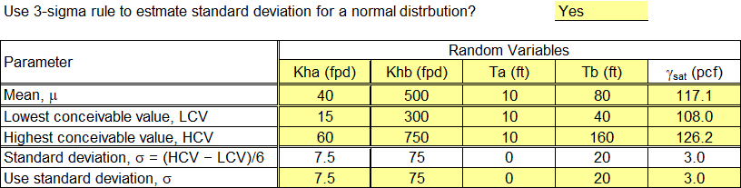
Step 1 characterizes the foundation. The input includes the saturated unit weight of the landside top stratum (γ_sat) and up to four additional random variables (e.g., thickness of top stratum, horizontal permeability of pervious foundation, permeability ratio, etc.). Normal distributions represent the random variables, and the mean (μ) and standard deviation (σ) are input.

The 3-sigma rule is based on the normal distribution probability density function, where the lowest conceivable value is about three standard deviations (3 sigma) below the mean, and the highest conceivable value is about three standard deviations above the mean. For the mean plus or minus three standard deviations (μ ± 3*σ), 99.73 percent of the area under the normal distribution is included. Therefore, 99.73 percent of all possible values of the random variable are included in the range of 6σ* (the highest possible value to the lowest possible value of the random variable). Thus, the standard deviation using the 3-sigma rule using Equation.

$$\sigma = \frac{HCV-LCV}{6}$$

where:

HCV = the highest conceivable value of the random variable
LCV = the lowest conceivable value of the random variable

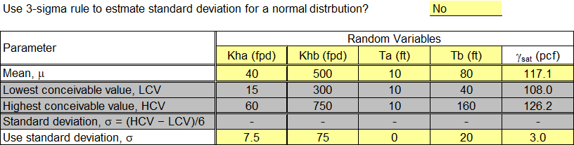
Use the drop-down list to select whether to use the 3-sigma rule to calculate the standard deviation of the random variables. For “Yes,” input the lowest conceivable value (LCV) and highest conceivable value (HCV). Although the standard deviation is calculated using the 3-sigma rule, it informs the user-specified value in the subsequent row, which is used in the calculations. For “No,” the standard deviation of the random variables is user-specified. Cells that do not apply have a gray background. These cells are not used in subsequent calculations even if data is present. The two possible scenarios are illustrated in Figure and Figure.

Figure: Step 1 of FOSM reliability worksheet: Input for standard deviation using 3-sigma rule.

Figure: Step 1 of FOSM Reliability Analysis worksheet: Input for standard deviation without using 3-sigma rule.

Reliability Analysis

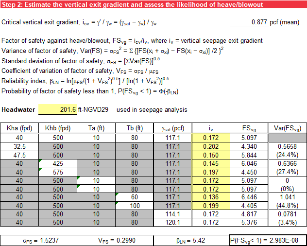
Step 2 calculates the critical vertical seepage exit gradient for heave/blowout (i_cv) using Equation.

$$i_{cv} = \frac{\gamma '}{\gamma_{w}} = \frac{\gamma_{sat}-\gamma_{w}}{\gamma_{w}}$$

where:

γ′ = submerged unit weight of the landside blanket
γ_sat = saturated unit weight of the landside blanket
γ_w = unit weight of water

The factor of safety against heave/blowout (based on vertical seepage gradients) (FS_vg) is calculated using Equation.

$$FS_{vg} = \frac{i_{cv}}{i_v}$$

where:

i_v = vertical seepage exit gradient

FS_vg represents an upper bound for an intact blanket (top stratum), and initiation occurs at significantly lower values in many cases through defects in the blanket (such as the data from Turnbull and Mansur for the lower Mississippi River).

The variance of the factor of safety against heave/blowout (Var[FS_vg]) is calculated using Equation.

$$Var[FS_{vg}] = \sigma^{2}_{FS_{vg}} = \sum_{i=0}^{n}[\frac{FS_{vg}(x_{i}+\sigma_{x_i}) - FS_{vg}(x_{i}-\sigma_{x_i})}{2}]^2$$

where:

n = number of random variables

The Var[FS_vg] for each random variable divided by the sum of all the variances gives the percentage that random variable affects the analysis. Thus, the random variable(s) that control(s) the reliability analysis can easily be determined based on the higher percentages. The relative contribution to the analysis is shown as a percentage beneath the Var[FS_vg] for each random variable.

The standard deviation and coefficient of variation of the FS_vg are calculated using Equation and Equation.

$$\sigma_{FS_{vg}} = \sqrt{Var[FS_{vg}]}$$

$$V_{FS_{vg}} = \frac{\sigma_{FS_{vg}}}{\mu_{FS_{vg}}}$$

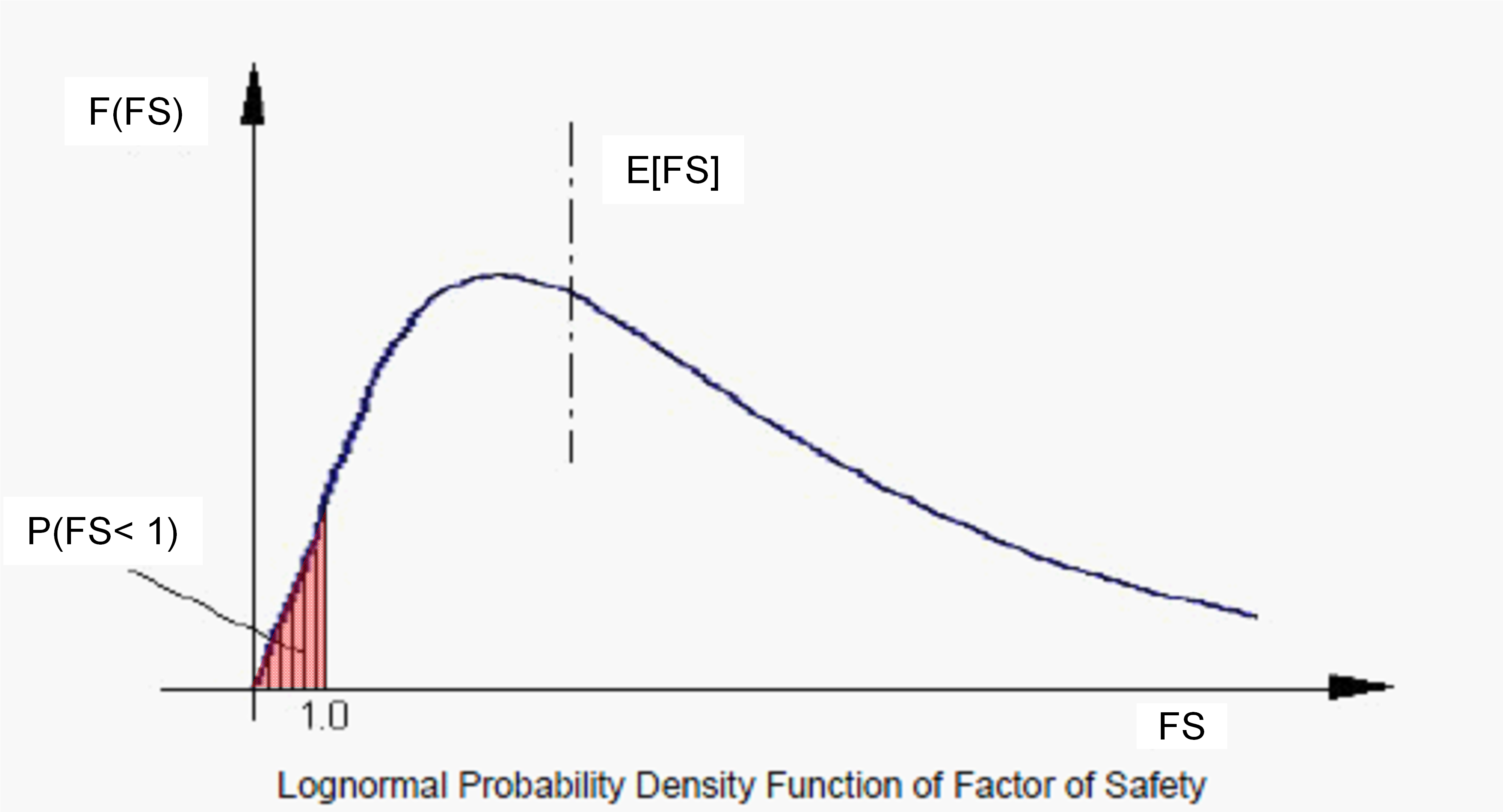
Physical quantities that result from a summation of many independent processes have distributions that are approximately normal. Physical quantities resulting from a product of many independent processes have distributions that are approximately lognormal. Lognormal distributions are used with reliability analyses. The probability density function of a factor of safety can be represented by a lognormal probability density function.

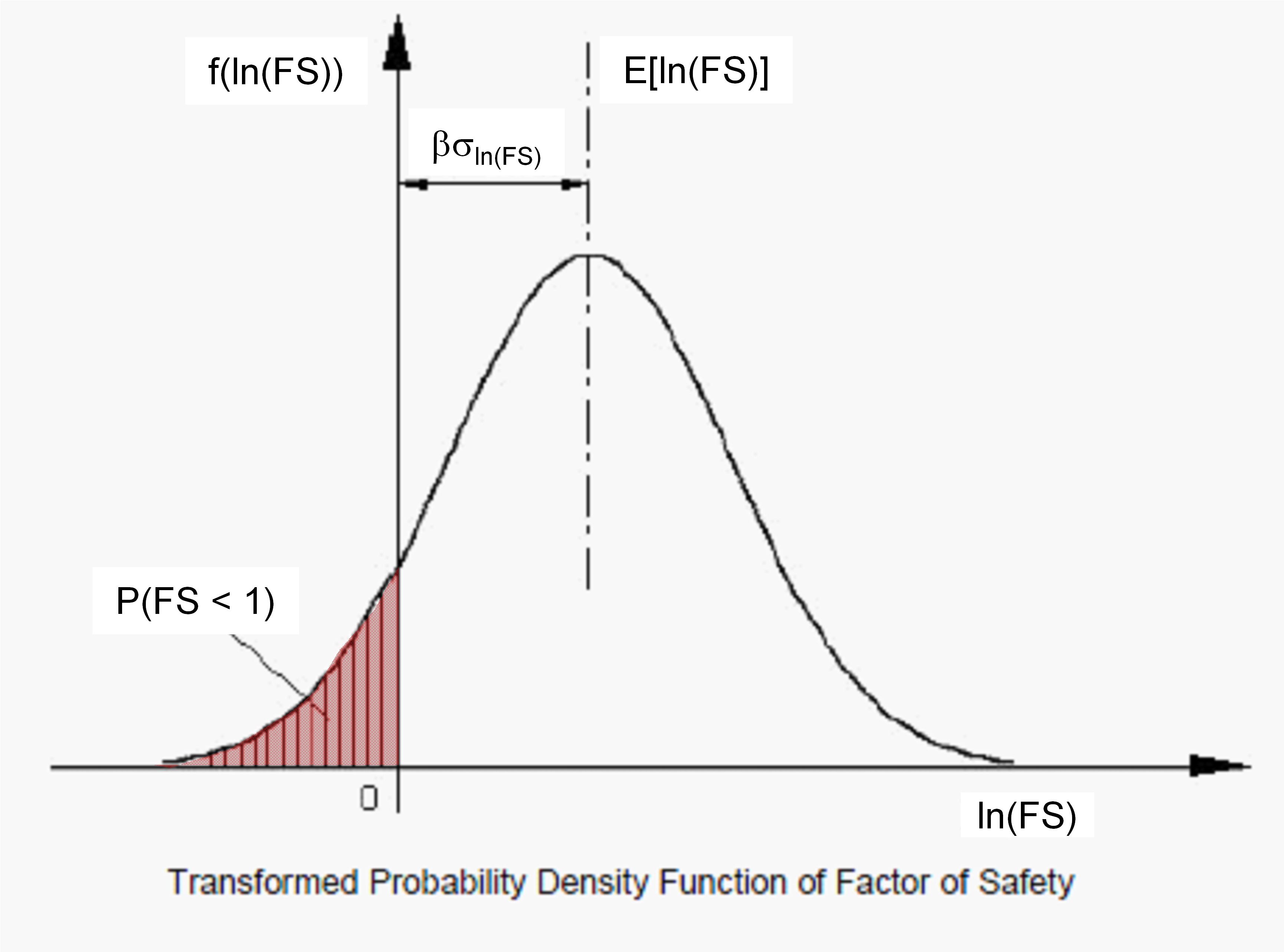
In Figure, the hatched area under the curve and to left of a FS of 1 gives the probability of a FS less than 1, P(FS < 1), often referred to as the probability of unsatisfactory performance, P(u), in reliability analysis. When the lognormal distribution is transformed to a normal distribution by taking the natural logarithm of the factor of safety, ln(1) = 0. Thus, P(FS < 1) is represented by the hatched area under the normal distribution curve to the left of zero in Figure.

Figure: Lognormal probability density function of factor of safety (ETL 1110-2-561).

Figure: Transformed probability density function of factor of safety (ETL 1110-2-561).

Lognormal is favorable for FS for several reasons. First, a lognormal function is never negative, and the FS is never negative. Second, the product of several variables is lognormally distributed.

The reliability index (β) is a measure of the distance that the mean of the FS is away from 1 or unsatisfactory performance. The larger the value of β, the more reliable the structure is for the performance mode being assessed (for example, seepage or stability). The smaller the value of β, the closer the condition is to unsatisfactory performance. The reliability index (b) is calculated using Equation.

$$\beta_{ln(FS_{vg})} = \frac{\ln( \frac { \mu_{FS_{vg}} } {\sqrt {1 + V_{FS_{vg}}^2 } })} {\sqrt{\ln(1+V_{FS_{vg}}^2)} }$$

The probability of a factor of safety against heave/blowout (based on vertical seepage gradients) less than 1 is calculated using Equation.

$$P(FS_{vg}<1) = \Phi(-\beta_ln(FS_{vg}))$$

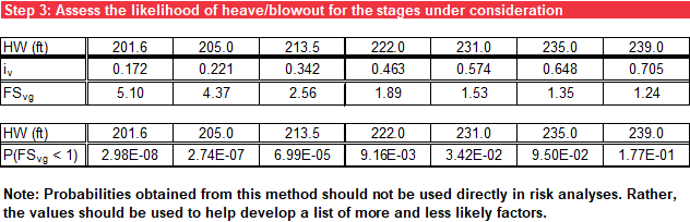
For each headwater level evaluated in the seepage analysis, the probability of a factor of safety against heave/blowout less than 1, P(FS_vg < 1), is calculated as shown in the example in Figure. The headwater input for these tables must be the headwater used in the seepage analysis, which can differ from the headwater levels input at the top of the worksheet. Do not include the headwater level where i_v = 0 in step 2 to avoid unexpected interpolation errors in step 3.

Figure: Step 2 of FOSM Reliability Analysis worksheet: Calculations based on seepage analysis results.

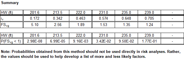
At the end of step 2, the mean factor of safety against heave/blowout and the probability of a factor of safety less than 1 are summarized as illustrated in Figure.

Figure: Step 2 of FOSM Reliability Analysis worksheet: Tabular output based on seepage analysis results.

Likelihood of Heave/Blowout at Landside Toe

Step 3 interpolates the mean factor of safety against heave/blowout (based on vertical seepage gradients) and the probability of a factor of safety less than 1 from the results of the seepage analysis for the headwater levels input at the top of the worksheet. The mean FS_vg values are linearly interpolated, and the P(FS_vg < 1) is interpolated using logarithmic scale for probability and linear scale for headwater as illustrated in Figure.

Figure: Step 3 of FOSM Reliability Analysis worksheet: Tabular output based on selected headwater levels.

Summary plots are generated after the tabular output. The first plot is the mean FS against heave/blowout (red solid line) and vertical seepage exit gradient at the landside levee toe (green solid line) as functions of headwater level. FS_vg is plotted on the primary y-axis, and i_v is plotted on the secondary y-axis. Horizontal reference lines display for the mean critical vertical seepage exit gradient (green dashed line) and factor of safety of 1 (red dashed line).

Figure illustrates the graphical deterministic output.

Figure: Step 3 of FOSM Reliability Analysis worksheet: Graphical output.

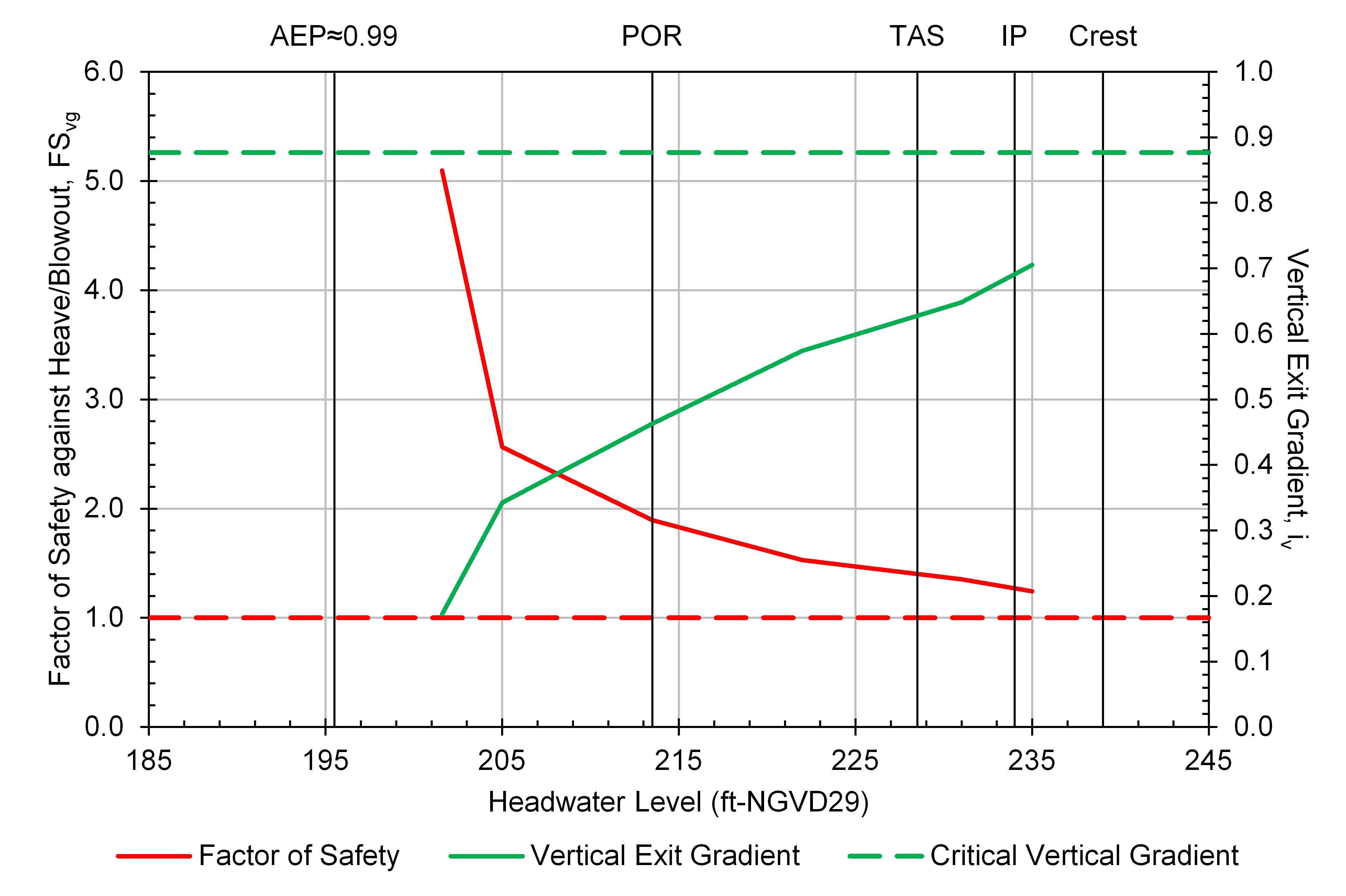
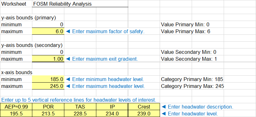
Figure illustrates the plot options for this chart. The maximum value for the primary y-axis (FS_vg), maximum value for the secondary y-axis (i_v), and minimum and maximum values for the x-axis (headwater level) are user-specified. Users can input up to five vertical reference elevations, and user-specified labels display at the top of the chart.

Figure: Step 3 of FOSM Reliability Analysis worksheet: Plot options for deterministic graphical output.

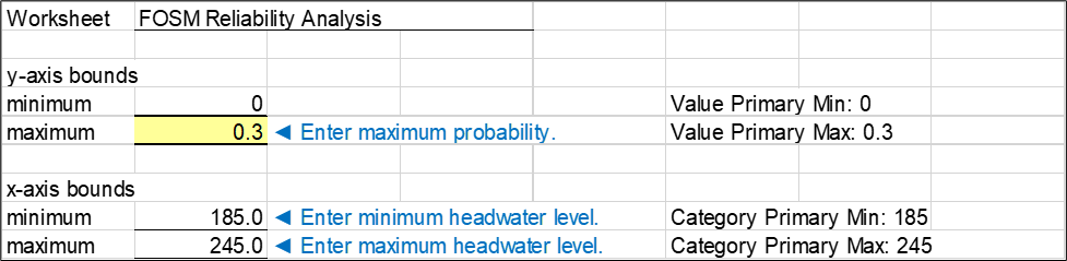
The mean probability of heave/blowout at the landside levee toe is plotted as a function of headwater level. Figure illustrates the graphical output for probabilistic analysis.

Figure: Step 3 of FOSM Reliability Analysis worksheet: Probabilistic graphical output.

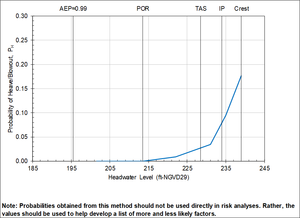
Figure illustrates the plot options for this chart. The vertical reference elevations and minimum and maximum values for the x-axis (headwater level) are the same as the input in Figure. Only the maximum value for the y-axis (probability of heave/blowout) is user-specified.

Figure: Step 3 of FOSM Reliability Analysis worksheet: Plot options for probabilistic graphical output.