11 Risk Analysis Results
Three tabs provide different views of the risk analysis results: the Loss Exceedance Plot, Conditional Loss Plot, and Summary Statistics tabs (Figure 11.1). The first two tabs display the risk analysis results graphically, while the last presents results in tabular form.

Figure 11.1: Risk results tabs.
Each risk result tab includes options to filter the results. To filter results, click the button next to Filter Results near the top of the tab. Use the checkboxes (Figure 11.2) to select which risk components and types to display in both graphical and tabular results. Risk components include the overall system, all system components, and all failure modes within each component.
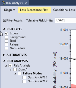
Figure 11.2: Select checkboxes for risk type and the system component in the graphical and tabular risk results.
RMC-TotalRisk reports five types of risk:
Excess Risk: Represents the increase in system risk due to failure, calculated using the probability of the hazard, the probability of failure, and the excess consequences. Excess consequences refer to the additional losses or damages caused by failure, beyond those that would occur during the same event if the structure did not fail.
Background Risk: Represents the risk assuming no structural flaws or vulnerabilities in the system. It reflects the risk from hazards alone, assuming there is no possibility of failure.
Total Risk: Represents the overall risk of the system (or component) and is calculated as the sum of failure risk and non-failure risk. Some USACE publications refer to total risk as residual risk (i.e., the risk that remains) [2] [9]. Proper estimation considers all relevant hazard sources, their likelihoods of occurrence, and their potential consequences. In this context, total does not necessarily mean that all potential sources of risk have been included.
Failure Risk: Represents the risk associated with system failure, calculated based on the probability of the hazard, the probability of failure, and the consequences of failure.
Non-Failure Risk: Represents the risk associated with the system not failing, calculated using the probability of the hazard, the probability of non-failure, and the consequences of non-failure. Infrastructure such as dams and levees often incurs consequences even when it does not fail. For example, during a major flood event, a dam might activate its emergency spillway, preventing the dam from reducing downstream flooding.
Dam and levee risk assessments often emphasize a limited range of flood and seismic hazard levels that could lead to failure, potentially overlooking the broader range of hazard levels that result in non-failure consequences. To accurately estimate background, non-failure, and total risk, it is essential to account for the full spectrum of hazard levels with adequate resolution.
For a detailed explanation of the underlying mathematics for the five types of risk, refer to the technical reference manual [1].
The following subsections describe the contents and functionality of each of the three risk results tabs.
11.1 Loss Exceedance Plot
The Loss Exceedance Plot displays consequences on the x-axis and the exceedance probability on the y-axis. This type of plot is commonly referred to as an F-N curve, survival function, or Farmer’s diagram [10]. If the hazard function is defined with annual exceedance probabilities, the y-axis of the loss exceedance plot will also represent annual exceedance probabilities. A log-log scale is typically used due to the wide range of probabilities and consequences, often spanning multiple orders of magnitude.
Figure 11.3 shows an example loss exceedance plot. After simulating risk with full uncertainty, the plot includes a 90% confidence interval shaded in red, along with the mean and median curves. By default, the USACE tolerable risk limit is displayed as a dotted black line [9]. You can customize this tolerable risk limit (TRL), also referred to as a guideline, or remove it from the plot as needed.
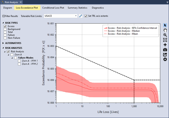
Figure 11.3: Example of Loss Exceedance Plot results with confidence intervals and the USACE tolerable risk limit.
To customize the TRL, select an option from the Tolerable Risk Limits dropdown menu(Figure 11.4). Available options include None, USACE, ANCOLD (2022 guidance), or a custom limit. To automatically set the plot extents to match the selected TRL extents, check the Set TRL axis extents checkbox.
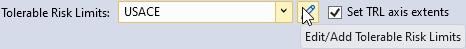
Figure 11.4: Tolerable risk guideline viewing options for graphical risk results in RMC-TotalRisk.
To add or edit custom limits, click the Edit/Add Tolerable Risk Limits button to open the Tolerable Risk Limit Editor (Figure 11.5).
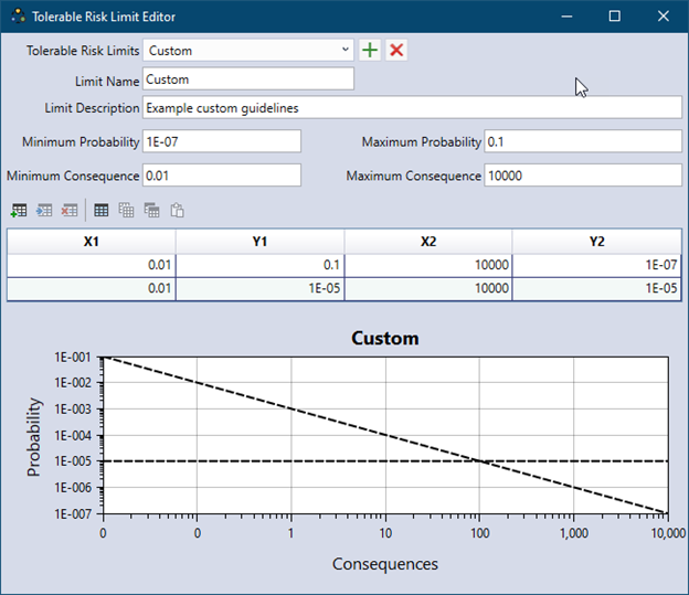
Figure 11.5: Tolerable Risk Limit Editor.
11.2 Conditional Loss Plot
USACE dam and levee safety programs commonly use the Conditional Loss Plot to display excess risk. In this plot, the conditional mean consequences are shown on the x-axis, and the probability of failure is shown on the y-axis. Similar to the Loss Exceedance Plot, a log-log scale is typically used due to the wide range of probabilities and consequences, which can span multiple orders of magnitude.
Traditionally, USACE refers to this plot as the \(f \cdot \overline{N}\) plot (pronounced as “little f-N bar” to distinguish it from the “big F-N” plot). However, in probability and statistics, \(f\) typically represents the probability density function, not exceedance probability. To avoid confusion and align with conventions in other disciplines, RMC-TotalRisk does not use the \(f \cdot \overline{N}\) notation for this plot. Users can, however, customize the plot axis labels if desired.
The Conditional Loss Plot is available only for failure risk and excess risk, as these risk types share the same probability of failure. Total risk and background risk are unconditional expectations where the total probability equals 1. Non-failure risk is a conditional expectation, where the total probability of non-failure equals 1 minus the probability of failure. However, since the probability of non-failure is typically very close to 1, this type of plot is not meaningful for non-failure risk.
Figure 11.6 shows a Conditional Loss Plot after simulating risk with full uncertainty. Uncertainty is visualized as a scatter cloud, which is thinned to a maximum of 1,000 points per system risk component for clarity. A red diamond indicates the mean excess risk result for the overall system. In this example:
The mean annual probability of failure is \(8.8\times10^{-6}\)
The conditional mean excess consequence is \(131.5\).
Stated differently, the mean annual probability of failure is \(8.8\times10^{-6}\), and if the system were to fail, the expected excess life loss would be \(131.5\).
The diagonal line on the plot represents the product of the probability of failure and the conditional mean excess loss, which equals the mean excess loss, \(\mathbb{E}[C]=1.2\times10^{-3}\). This value plots slightly above the tolerable risk limit of \(1\times10^{-3}\).
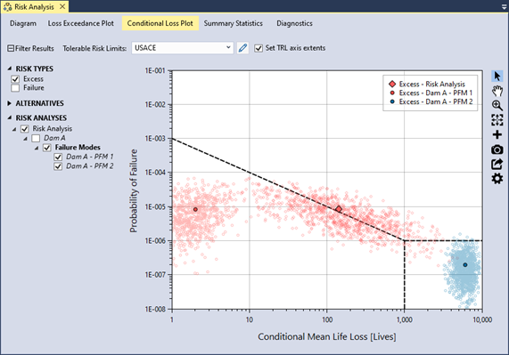
Figure 11.6: Conditional Loss Plot displaying excess risk results as the probability of failure and the conditional mean life loss, showing USACE Tolerable Risk Limits as dotted black lines.
11.3 Summary Statistics
The Summary Statistics tab displays result statistics for each of the filtered risk measures (Figure 11.7).
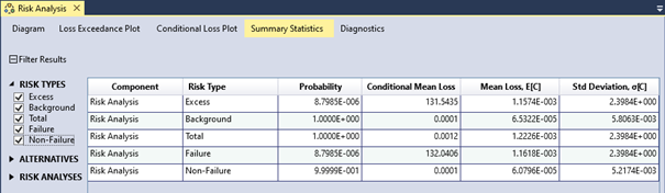
Figure 11.7: Risk analysis results on the Summary Statistics tab in RMC-TotalRisk.
Component: This column identifies the overall system by the name of the risk analysis. System components use the name of the selected hazard function by default, and failure modes are labeled with the system component name and the selected response function.
Risk Type: This column lists the five types of risk that RMC-TotalRisk reports (excess, background, total, failure, and non-failure).
Probability: This column shows the total probability for the risk type. For excess and failure risk, it represents the probability of failure. For background and total risk, the probability is always 1. For non-failure risk, it is 1 minus the failure probability, which is typically very close to 1.
Conditional Mean Loss: This column displays the mean (or expected) consequences given system failure. The product of probability and conditional mean loss equals the unconditional mean loss, \(\mathbb{E}[C]\). This measure is most relevant for excess and failure risk, where the probability of failure is explicitly considered. For background and total risk, the conditional mean equals the unconditional mean.
Mean Loss, Ε[C]: This column shows the mean (or expected) consequences, calculated as a probability-weighted average over all hazardous events. In flood damage assessments, this value is commonly called Expected Annual Damage (EAD). In USACE dam and levee safety programs, it is referred to as Average Annual Life Loss (AALL).
Standard Deviation, σ[C]: This column presents the standard deviation of the consequences, which measures deviation from the mean loss. When comparing two risk reduction alternatives with the same mean loss, the option with the smaller standard deviation is considered less risky.