12 Risk Analysis Diagnostics
RMC-TotalRisk includes several diagnostic tools to help explore the Monte Carlo simulation results for a risk analysis with full uncertainty. These diagnostics are most useful when the risk analysis inputs include uncertainty. If no uncertainty is defined, the diagnostic tools have limited applicability. The following subsections describe the available risk analysis diagnostics.
12.1 Integration
The integration diagnostics estimate the standard error of the computed total risk for the system and report the number of integrand function evaluations performed during the risk simulation. These diagnostics are displayed graphically as a kernel density or cumulative distribution plot. A table summarizes key statistics, including the mean, standard deviation, and key percentiles.
Figure 12.1 shows an example of the integration diagnostics for the estimated integration standard error during the simulation. In this example, the integration standard error averaged \(5.4×10^{-7}\) for each Monte Carlo realization.
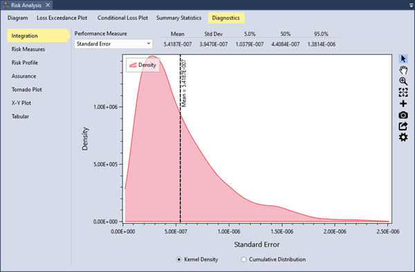
Figure 12.1: Example of integration diagnostics.
12.2 Risk Measures
RMC-TotalRisk computes seven risk measures for each of the five risk types:
Probability: Represents the total probability of the risk type. For excess and failure risk, this is the probability of failure. For background and total risk, the probability is 1. For non-failure risk, it is 1 minus the failure probability, which is typically very close to 1.
Conditional Mean Loss: Represents the mean (or expected) consequences given system failure. The product of probability and conditional mean loss equals the mean loss, \(\mathbb{E}[C]\). This measure is most applicable for excess and failure risk, where the probability of failure is explicitly considered. For background and total risk, the conditional mean equals the unconditional mean.
Mean Loss, Ε[C]: Represents the mean (or expected) consequences, calculated as a probability-weighted average over all hazardous events. In flood damage assessments, this term is commonly called Expected Annual Damage (EAD). In USACE dam and levee safety programs, it is referred to as Average Annual Life Loss (AALL).
Standard Deviation, σ[C]: Represents the standard deviation of the consequences, which measures deviation from the mean loss. When comparing two risk reduction alternatives with the same mean loss, the option with the smaller standard deviation is considered less risky.
Consequence Threshold Probability: Represents the probability of exceeding a user-specified consequence threshold. For example, you might calculate the probability of exceeding a life loss of 10 lives.
Value-at-Risk (VaR): Represents the minimum consequences for a user-specified exceedance probability \(\alpha = 0.01\). By default, RMC-TotalRisk calculates the minimum consequences occurring during a 100-year event (alpha = 0.01).
Conditional Value-at-Risk (CVaR): Represents the conditional mean (or expected) consequences for a user-specified exceedance probability \(\alpha\). By default, RMC-TotalRisk calculates the expected consequences for all events equal to or larger than a 100-year event (\(\alpha = 0.01\)).
For mathematical details on these risk measures, refer to the technical reference manual[1].
As shown in Figure 12.2, you can select the desired risk type and risk measure from the dropdown menus to view the results.
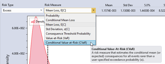
Figure 12.2: Select the risk type and risk measure to display results.
You can display the distribution as either a kernel density plot or a cumulative distribution plot using the radio buttons at the bottom of the plot. Summary statistics for the distribution appear in the upper right-hand corner (Figure 12.3).
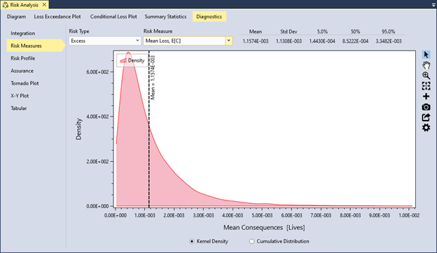
Figure 12.3: Risk measure diagnostic tools in RMC-TotalRisk showing the kernel density of the excess mean loss, E[C].
12.3 Risk Profile
A risk profile plots exceedance probabilities or conditional mean loss against increasing hazard levels. You can filter the risk profile results by system component and risk type. This plot helps identify critical hazard levels where the probability of failure or risk increases sharply.
Figure 12.4 shows the hazard exceedance probability for the background risk at Dam A. Since background risk represents the residual risk from the natural hazard, this risk profile aligns with the input reservoir stage-frequency hazard function.
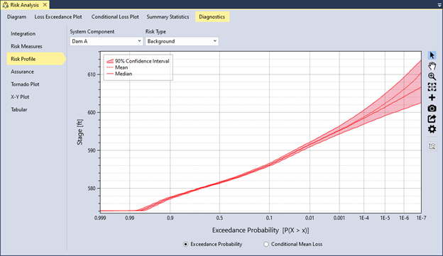
Figure 12.4: Example of a risk profile plot showing the hazard exceedance probability for the background risk at Dam A.
Figure 12.5 displays the hazard exceedance probability for the excess risk at Dam A. The profile shows an inflection point near a reservoir stage of 595 feet. This inflection occurs because Potential Failure Mode 1 (spillway erosion) has a nonzero probability of failure beginning at this hazard level. At this point, excess risk starts to increase.
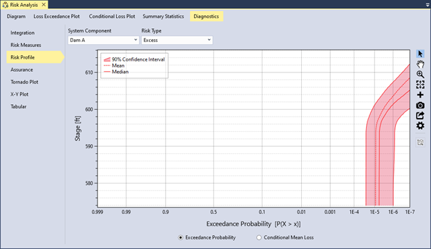
Figure 12.5: Example of a risk profile plot showing the hazard exceedance probability for the excess risk at Dam A.
12.4 Assurance
RMC-TotalRisk provides an assurance plot and summary statistics based on a user-defined profile hazard type and hazard threshold. This diagnostic supports the National Flood Insurance Program (NFIP) for levees. For more details, refer to the technical reference manual [1].
Figure 12.6 illustrates an example risk diagram for a levee risk analysis. The primary hazard is river peak flow frequency, which is transformed into a peak river stage using a flow-to-stage rating curve derived from a hydraulic routing model. Potential Failure Modes (PFMs) include a Prior OT failure mode from backward erosion piping and an OT failure mode. The top of the levee is at a river stage of 65 feet.
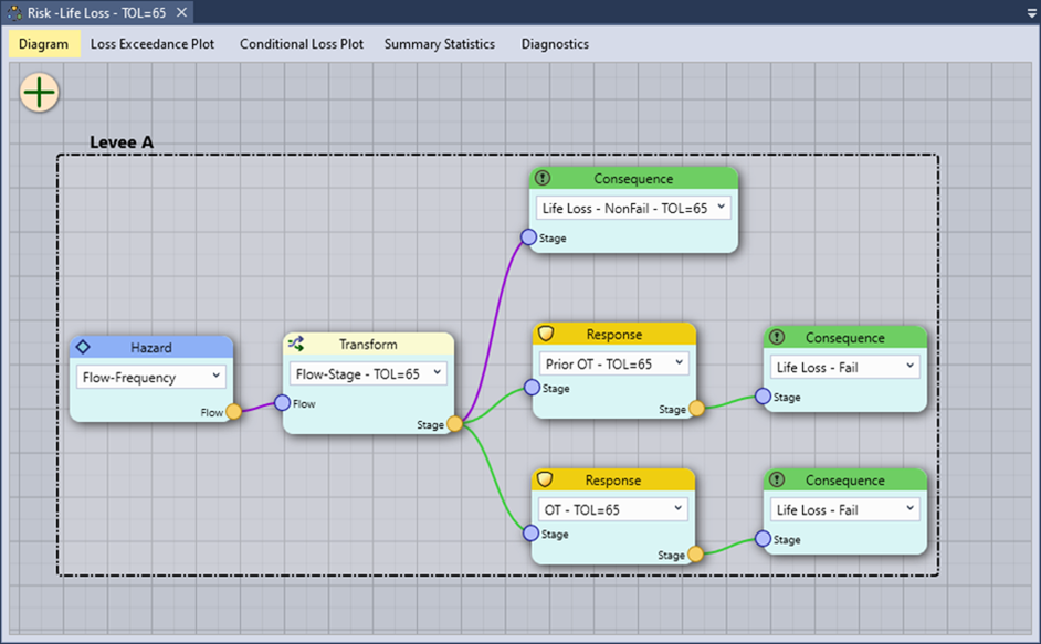
Figure 12.6: Example risk diagram for a levee risk analysis.
To compute assurance, select the profile hazard type and specify the hazard threshold for the desired system component in the risk analysis options, as shown in Figure 12.7.
Profile Hazard: This option sets the hazard function used to construct risk profiles and estimate the probability of exceeding a hazard threshold. You can select the primary hazard function or any hazard-to-response transform functions. For levee accreditation analyses, use stage or water surface elevation as the profile hazard type.
Hazard Threshold: This setting defines the hazard level for calculating the probability of exceeding that threshold. The default hazard threshold is 0. For levee accreditation analyses, use the top of levee stage or elevation as the hazard threshold.
The assurance diagnostic estimates the uncertainty in the annual probability of inundation (API). The level of assurance (e.g., 85% assurance for levee accreditation) corresponds to the confidence level of the API (e.g., the leveed area is inundated with a probability of 0.01 or less with 85% confidence). To assess assurance using RMC-TotalRisk, simulate the risk analysis with full uncertainty.
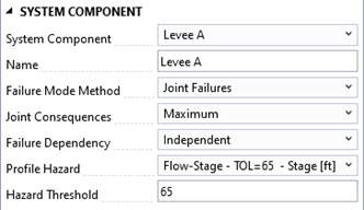
Figure 12.7: Setting the profile hazard type and threshold level for the system component.
After completing the risk analysis, navigate to the Diagnostics tab and select Assurance. The plot includes the following features:
The API is plotted on the x-axis, while the non-exceedance probability of API uncertainty is on the y-axis.
The mean API is represented by a vertical dashed blue line.
If the assurance level is less than 65%, the target level line is a vertical red line.
For assurance between 65% and 85%, the target level line is orange.
Assurance levels above 85% are indicated by a green line.
Figure 12.8 shows the standard cumulative distribution plot for assurance in the levee risk analysis example. The mean API is 0.00647, and the target level of 0.01 (100-year) has an assurance level of 84.6%, represented by the orange line. Since the assurance level falls between 65% and 85%, the levee accreditation recommendation must be supported by uncertainty analysis, past system performance, and other factors [11].
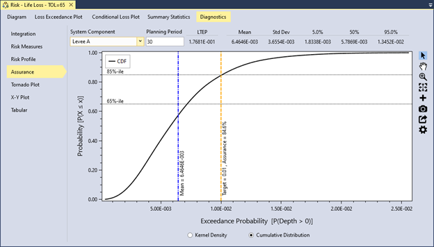
Figure 12.8: Example of the cumulative distribution plot for NFIP assurance.
12.5 Tornado Plot
A tornado plot (Figure 12.9) visually illustrates the sensitivity of risk results to input functions at each hazard level. The plot is based on the selected system component, risk type, sensitivity measure, and hazard level. Inputs are ranked from most sensitive at the top to least sensitive at the bottom. Sensitivity measure options include Sensitivity Index, Pearson’s Correlation, and Spearman’s Correlation.
Risk sensitivity often varies with hazard level. For instance, at low hazard levels, the results might be most sensitive to uncertainty in the system response, while at higher hazard levels, they may become more sensitive to uncertainty in the hazard probability. You can adjust the hazard level by moving the slider next to the hazard level text box to explore how component sensitivity changes across the range of hazard levels.
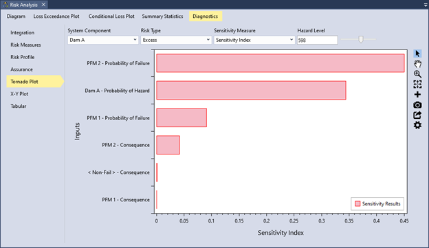
Figure 12.9: Example of a tornado plot for risk diagnostics.
12.6 X-Y Plot
The X-Y plot evaluates the correlation between different system risk components and inputs. You can filter results by risk type, risk measure, X parameter, and Y parameter components. For example, you might set the overall risk of failure at the dam as the Y parameter and the risk of failure from an individual failure mode as the X parameter.
In the dam risk example (Figure 12.10), the X-Y plot reveals a strong correlation between the excess risk of failure mode PFM 2 (concentrated leak erosion) and the excess risk of the overall system; i.e., the system risk is dominated by PFM 2. This indicates that significant changes in the PFM 2 failure mode correspond to substantial changes in overall system risk. These findings are consistent with the sensitivity results shown in Figure 12.9.
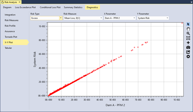
Figure 12.10: Example of a X-Y plot for risk diagnostics.
12.7 Tabular
Tabular results display data based on the selected risk type and risk measure (Figure 12.11). The table includes a column for each system component and a row for each Monte Carlo realization. Use the table column tools to export, copy, or analyze the data.
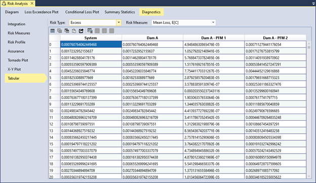
Figure 12.11: Tabular diagnostics tab displays every Monte Carlo realization for the selected risk type and risk measure.
To analyze a specific column, right-click on the column header and select Summary Statistics…. This action generates a histogram plot and detailed summary statistics for the selected column, as shown in Figure 12.12.
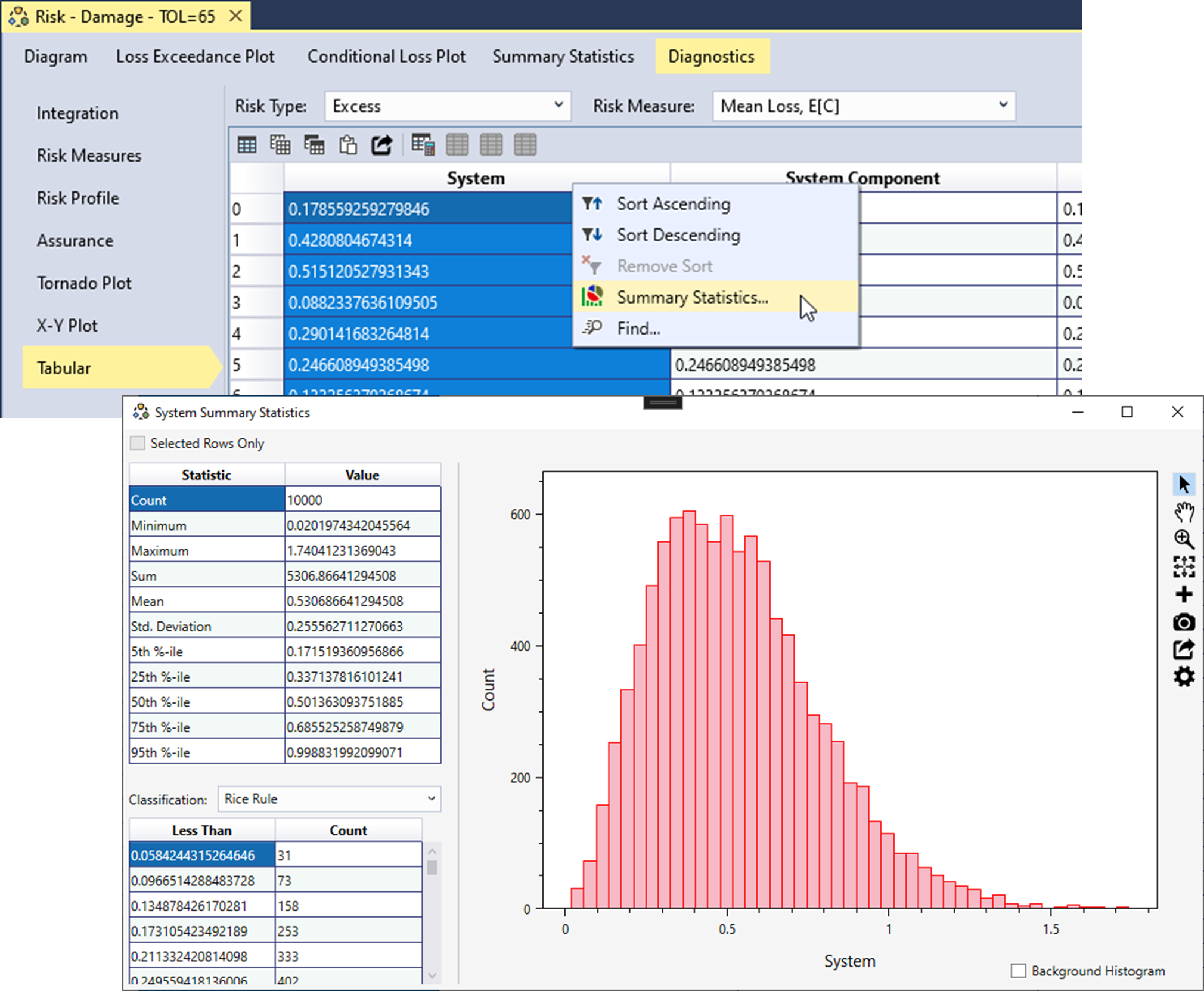
Figure 12.12: Example of the histogram and summary statistics output for tabular results.