6 Hazard Functions

RMC-TotalRisk defines a hazard function by the exceedance probabilities of various hazard levels, such as annual maximum peak flow or WSE. Hazard functions are also commonly referred to as frequency curves. In dam and levee risk assessments, the annual maximum peak WSE (or stage) or the annual maximum peak ground acceleration are typically the primary hazard parameters for evaluating a potential failure mode [3] [4]. As such, the hazard functions commonly describe the annual exceedance probability (AEP) of these hazard levels.

RMC-TotalRisk provides six options for adding a hazard function: import from RMC-BestFit, import from RMC-RFA, or creating a parametric, nonparametric, tabular, or composite function. The following subsections explain each option in detail.

6.1 Import from RMC-BestFit

The USACE RMC, in collaboration with the Engineer Research and Development Center (ERDC) Coastal and Hydraulics Laboratory (CHL), developed the Bayesian estimation and fitting software (RMC-BestFit) to enhance and expedite flood hazard assessments within the Flood Risk Management, Planning, and Dam and Levee Safety communities of practice [5]. You can download RMC-BestFit from the RMC Website. RMC-TotalRisk allows you to directly import results from an RMC-BestFit version 1.0 analysis.

To import results of an RMC-BestFit analysis, right-click on the Hazards folder in the Project Explorer (Figure 6.1) or navigate to Project Menu > Hazards and select Add RMC-BestFit Hazard…. When the dialog appears, enter the name of the hazard function, choose the RMC-BestFit project file, and select the Bayesian analysis you want to import.

After finalizing the import settings, click OK (Figure 6.1). The RMC-BestFit hazard function is added to the Hazards folder in Project Explorer, the function opens into the Tabbed Documents area, and the input data properties display in the Properties window. From here, you can edit the name, description, hazard type, and hazard units as needed.

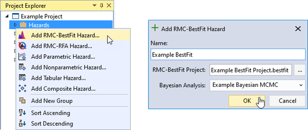
Figure 6.1: Add RMC-BestFit hazard function option and RMC-BestFit import dialog.

When you create a new RMC-BestFit hazard function, the system automatically sets the hazard type to Stage and the units to ft. To change these default settings, navigate to Tools > Options > Defaults. For more information, refer to section 4.8.

In the Properties window, use the dropdown menus to specify the hazard type and units (Figure 6.2). If the desired hazard type or unit is not listed, click the “plus” button to add a new option. To remove an option, click the X beside it in the dropdown. Once you define the hazard type and units, the hazard function is ready to use.

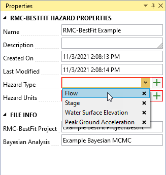
Figure 6.2: RMC-BestFit hazard function properties window.

6.1.1 Graphical Results

RMC-TotalRisk offers several tools to help you explore the results of a Bayesian analysis imported from RMC-BestFit. By default, the results open in the Graphical Results tab (Figure 6.3), displaying the posterior predictive (mean hazard), posterior mode, and Bayesian credible intervals (90% confidence).

The hazard function initially appears as a frequency curve, with exceedance probabilities plotted on the x-axis using a Normal scale and magnitude on the y-axis using a logarithmic scale. You can edit the plot properties, flip the axes, or adjust the axis scales as needed. RMC-TotalRisk automatically saves any changes you make to the plot.

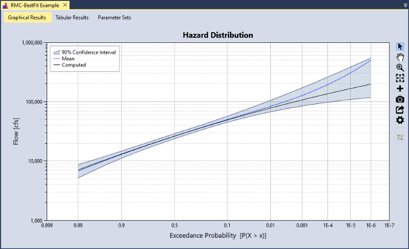
Figure 6.3: Graphical frequency results.

6.1.2 Tabular Results

Click the Tabular Results tab to view the frequency curve results and the posterior mode summary statistics, as shown in Figure 6.4.

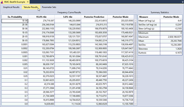
Figure 6.4: Tabular frequency results.

6.1.3 Parameter Sets

The Parameter Sets tab provides access to all output posterior parameter sets, as shown in Figure 6.5. You can sort the tables, copy the data, or export all values for external use.

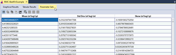
Figure 6.5: Parameter sets results.

You can also generate summary statistics for parameter set columns, such as the Mean (of log) (µ) column shown in Figure 6.6.

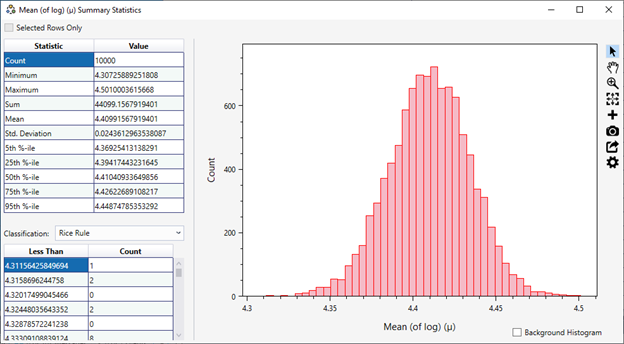
Figure 6.6: Summary statistics on parameter sets for mean (of log) (µ).

6.2 Import from RMC-RFA

The USACE RMC developed the Reservoir Frequency Analysis (RMC-RFA) software to facilitate hydrologic hazard assessments for the USACE Dam Safety Program. RMC-RFA produces a reservoir stage-frequency curve with uncertainty bounds by using a deterministic flood routing model while treating the inflow volume, the inflow flood hydrograph shape, the seasonal occurrence of the flood event, and the antecedent reservoir stage as uncertain variables rather than fixed values [4]. You can download RMC-RFA from the RMC Website. RMC-TotalRisk allows you to directly import results from an RMC-RFA version 1.1.0 analysis.

To import results of an RMC-RFA analysis, right-click on the Hazards folder in the Project Explorer (Figure 6.7) or go to Project Menu > Hazards and select Add RMC-RFA Hazard…. When the dialog appears, enter the name of the hazard function, select the RMC-RFA project file, choose the output type, and select the simulation you want to import.

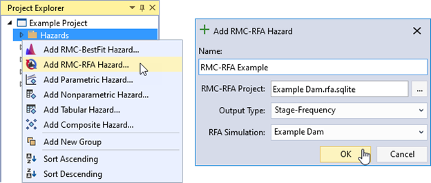
Figure 6.7: Add new RMC-RFA hazard function and import dialog.

After finalizing the import settings, click OK (Figure 6.7) and the RMC-RFA hazard function is added to the Hazards folder in Project Explorer. The function automatically opens into the Tabbed Documents area, and the Properties window displays the input data properties (Figure 6.8). From here, you can set the name, description, hazard type, hazard units, and hazard and probability interpolation transforms.

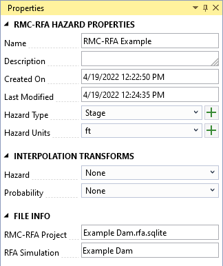
Figure 6.8: RMC-RFA hazard function properties.

Similar to the RMC-BestFit hazard function, you can view RMC-RFA results in either graphical or tabular form. For more details on these viewing options, refer to section 6.1.

6.3 Parametric Hazard Function

This option allows you to define a hazard function using a parametric distribution. To create a parametric hazard function, right-click on the Hazards folder in the Project Explorer (Figure 6.9) or go to Project Menu > Hazards and select Add Parametric Hazard…. Enter a name for the parametric hazard function and click OK.

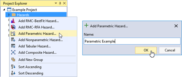
Figure 6.9: Create new parametric hazard function.

After creating the parametric hazard function, the system automatically opens it in the Tabbed Documents area and displays its properties in the Properties window (Figure 6.10). In the Properties window, you can set the name, description, hazard type, and hazard units. Define the parametric distribution with uncertainty by setting the effective record length (ERL), type of distribution, and parameters for the distribution. Uncheck the Uncertainty On checkbox to use the parametric function without uncertainty. Once the parameters have been set, click the Compute button to generate and view the parametric hazard function.

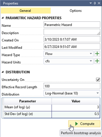
Figure 6.10: Parametric hazard function properties.

Additional options for computing the parametric function are available in the Options tab in the Properties window, including bootstrap sampling, confidence interval, number of realizations, a pseudo random number generator (PRNG) seed for random number generation, and output probability ordinates.

You can view the parametric frequency results in either graphical or tabular form. For more details on these viewing options, refer to section 6.1.

6.4 Nonparametric Hazard Function

This option lets you define a hazard function with a nonparametric distribution using tabular data, where the ERL determines the level of uncertainty. A longer ERL reduces uncertainty and narrows the confidence intervals. The most common use case involves copying and pasting a nonparametric frequency function from another application, such as Microsoft Excel, HEC-FDA, or HEC-SSP, and then entering the ERL to define uncertainty.

To create a nonparametric hazard function, right-click on the Hazards folder in the Project Explorer (Figure 6.11) or go to Project Menu > Hazards and select Add Nonparametric Hazard…. Enter a name for the nonparametric hazard function and click OK.

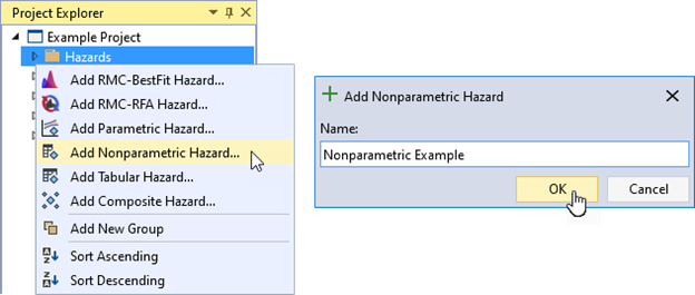
Figure 6.11: Create new nonparametric hazard function.

After creating the nonparametric hazard function, the system automatically opens it in the Tabbed Documents area and displays the tabular function properties in the Properties window (Figure 6.12). In the Properties window, you can set the name, description, hazard type, hazard units, hazard and probability interpolation transforms, ERL, and extrapolation probability. The interpolation transforms define how the data is interpolated when sampling values between the specified tabular ordinates. The ERL determines the level of uncertainty in the nonparametric function. The extrapolation probability input extrapolates a less frequent exceedance probability. If the user-defined data already extends beyond the entered value, no extrapolation occurs.

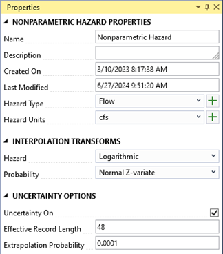
Figure 6.12: Nonparametric hazard function properties.

The Tabbed Document for a nonparametric function includes a table for data entry and a graphical representation of that data (Figure 6.13). You can manually enter data into the table or paste it from another source, such as Microsoft Excel.

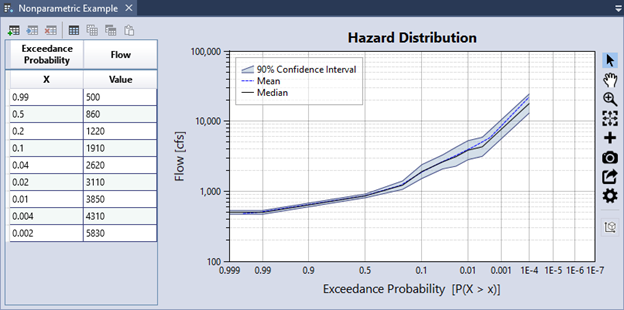
Figure 6.13: Nonparametric hazard function example.

6.5 Tabular Hazard Function

This option provides a straightforward way to define a hazard function using tabular data. The most common use case involves copying and pasting a frequency function from another application, such as Microsoft Excel or HEC-SSP.

To create a tabular hazard function, right-click the Hazards folder in the the Project Explorer(Figure 6.14) or go to Project Menu > Hazards and select Add Tabular Hazard…. Enter a name for the tabular hazard function and click OK.

Figure 6.14: Create new tabular hazard function.

After creating the tabular hazard function, the system automatically opens it in the Tabbed Documents area and displays its properties in the Properties window (Figure 6.15). In the Properties window, you can set the name, description, hazard type, hazard units, and hazard and probability interpolation transforms. The interpolation transforms define how the data is interpolated when sampling values between the specified tabular ordinates.

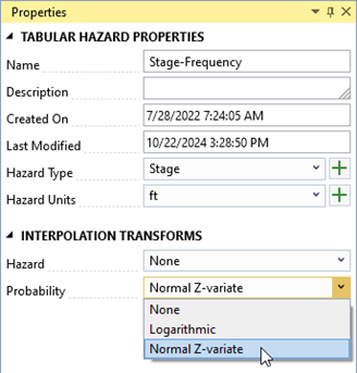
Figure 6.15: Tabular hazard function properties.

The Tabbed Document for a tabular hazard function contains a table for data entry and a graphical representation of the data (Figure 6.16). Define uncertainty around either the hazard or the probability by making a selection from the Uncertain Value dropdown in the top left of the document. Select a distribution to define uncertainty and enter parameters for the selected distribution for each ordinate in the tabular data. You can enter data manually into the table or paste it from another source, such as Microsoft Excel.

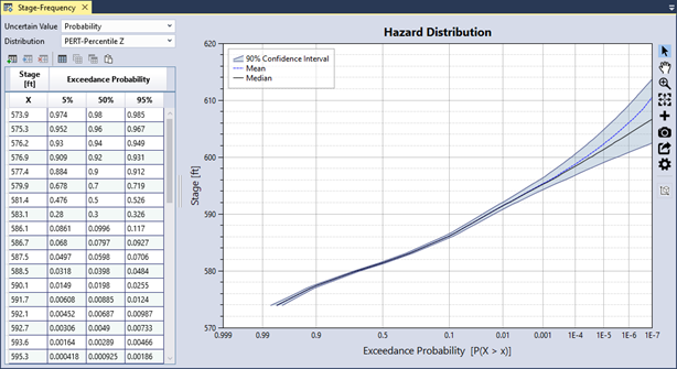
Figure 6.16: Tabular hazard function example.

6.5.1 Data Validation

The input data table has built-in validation. Tabular data must meet the following requirements:

• The hazard values must be in ascending order.

• The probability values must be in descending order, as they represent exceedance probabilities.

• If uncertainty is defined, the uncertain ordinates must contain valid distribution parameters, and the uncertainty bounds must be properly ordered.

• Probability values must be between 0 and 1.

If you enter invalid data, the corresponding table cell turns red, and a tooltip explains the error, as shown in Figure 6.17. Additionally, an error message appears in the Message window, prompting you to resolve all errors in the data table.

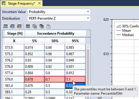
Figure 6.17: Tabular hazard input data validation.

6.6 Composite Hazard Function

This option allows you to combine multiple hazard functions into a single function by assigning weights to the individual input functions.

To create a composite hazard function, right-click on the Hazards folder in the Project Explorer (Figure 6.18) or go to Project Menu > Hazards and select Add Composite Hazard…. Enter a name for the composite hazard function and click OK.

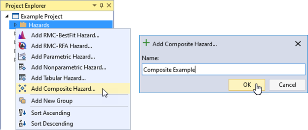
Figure 6.18: Create new composite hazard function.

When you create a new composite hazard function, it automatically opens in the Tabbed Documents area, and the Properties window displays the composite function’s properties (Figure 6.19). In the Properties window, you can set the name, description, hazard type, hazard units, and input hazard functions. Define the input functions in the Hazard functions table. Click the Add Row(s) button in the table toolbar to add rows for the input functions. Ensure that the weights assigned to the hazard functions sum to 1. If the hazard functions are competing, uncheck the Is Mixture checkbox and select a Dependency type: Independent, Perfectly Positive, or Perfectly Negative.

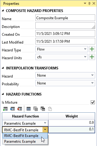
Figure 6.19: Composite hazard function properties.

The Tabbed Document for a composite function contains a graphical representation of the composite function (Figure 6.20).

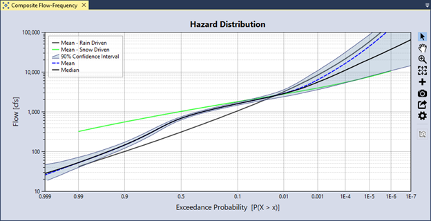
Figure 6.20: Composite hazard function graphical display.

References

[3]

Best practices in dam and levee safety risk analysis. Lakewood, CO: U.S. Department of the Interior, Bureau of Reclamation; U.S. Army Corps of Engineers, 2019. Available: https://www.usbr.gov/damsafety/risk/methodology.html

[4]

C. H. Smith, M. Bartles, and M. Fleming, “Hydrologic hazard methodology for semi-quantitative risk assessments,” U.S. Army Corps of Engineers, Institute for Water Resources, Risk Management Center, RMC-TR-2018-03, 2018. doi: http://dx.doi.org/10.13140/RG.2.2.11090.89288.

[5]

C. H. Smith and M. Daughty, “RMC-BestFit quick start guide,” U.S. Army Corps of Engineers, Institute for Water Resources, Risk Management Center, RMC-TR-2020-03, 2020. doi: http://dx.doi.org/10.13140/RG.2.2.23168.97280.