Internal Erosion Suite

Steel and Aluminum Pipes

Galvanized (zinc-coated), corrugated steel pipes (CSPs) are commonly used for gravity drainage structures in many levee embankments and floodwalls in the USACE portfolio. They are much less common in USACE dams because of significant structural loads acting on the pipe and high-flow velocities. They may be present in low-head dams. Corrugated aluminum pipes (CAPs) are also widely used, typically when potential corrosion causes concern from the soil surrounding the pipe or the effluent flowing through the pipe. Non-corrugated steel and aluminum pipes are used but much less frequently than corrugated pipes. This worksheet can assess both corrugated and non-corrugated steel and aluminum pipes.

Pipe Material and Shape Characterization

Step 1 characterizes the pipe material and shape. Select the pipe material using the drop-down list as shown in Figure. CSP galvanized with a protective zinc coating, aluminum-coated Type 2 CSP (ALCLAD® or equivalent), and aluminum-zinc alloy-coated CSP (Galvalume® or equivalent) can be evaluated.

Figure: Step 1 of Steel and Aluminum Pipe worksheet: Pipe material characterization.

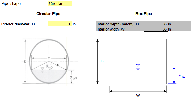
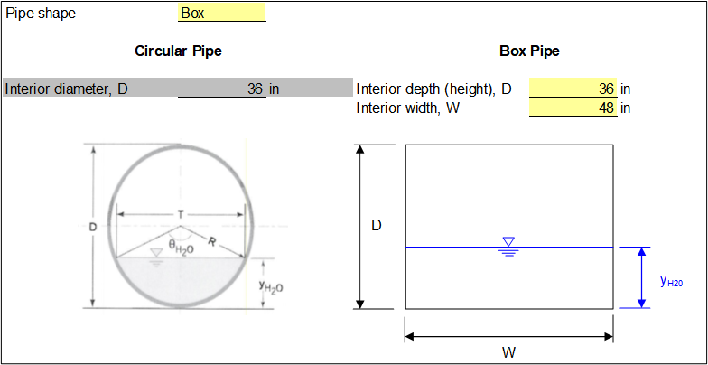
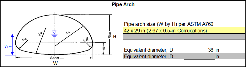
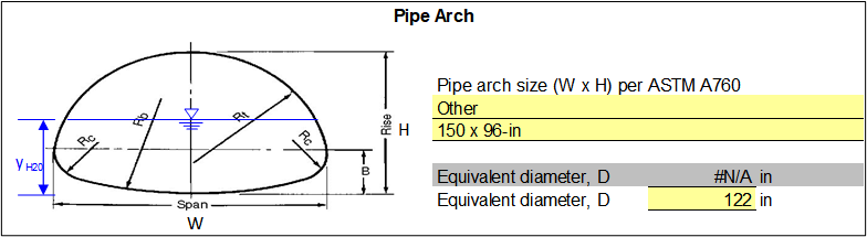
Select the pipe shape using the drop-down list as shown in Figure. Circular, box, and arch pipe can be evaluated. For Circular, specify the interior diameter as illustrated in Figure. For Box, specify the interior depth (height) and interior width as illustrated in Figure. For Arch, choose the pipe arch size based on American Society for Testing and Materials (ASTM) A760 from the drop-down list, and the equivalent diameter displays as illustrated in Figure. For Other for pipe arch size, specify the pipe arch size and equivalent diameter as illustrated in Figure. Cells that do not apply have a gray background.

Figure: Step 1 of Steel and Aluminum Pipe worksheet: Circular pipe dimensions.

Figure: Step 1 of Steel and Aluminum Pipe worksheet: Box pipe dimensions.

Figure: Step 1 of Steel and Aluminum Pipe worksheet: ASTM A760 arch pipe dimensions.

Figure: Step 1 of Steel and Aluminum Pipe worksheet: User-specified arch pipe dimensions.

Flow Velocity Characterization

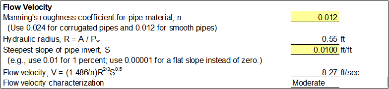
Step 2 uses Manning’s equation (Equation) to calculate the velocity (ft/sec) of flow through the pipe for significant (but not extreme) rainfall events.

$$V=\left(\frac{1.486}{n}\right)R^{2/3}S^{1/2}$$

where:

n = Manning's roughness coefficient for the pipe material
R = hydraulic radius of the pipe (ft)
S = steepest pipe invert slope (ft/ft)

Specify the Manning’s roughness coefficient (n). Various sources are available for n values, but in most cases, the pipe has either a corrugated or smooth interior flow surface. For pipes with an interior corrugated flow surface, the suggested value is 0.024. If the interior flow surface is smooth, the suggested value is 0.012 (USACE 2020) [?].

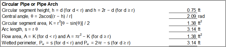
The hydraulic radius (R) is a function of the pipe shape and depth of flow, as calculated in Equation.

$$R = \frac{A}{P_w}$$

where:

A = cross-sectional area of the flow in the pipe (ft²)
P_w = wetted perimeter of the flow in the pipe (ft)

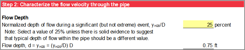
To obtain A and P_w, the depth of flow in the pipe during a significant (but not extreme) rainfall event ($y_{H2O}$) for each pipe shape is required. Instead of a selecting a flow depth, the flow depth is normalized with the interior pipe depth (height) from step 1. Select the normalized flow depth ($y_{H2O}/D$) using the drop-down list. Normalized flow depths of 100, 87.5, 75, 50, 25, 10, and 5 percent can be evaluated. If a pipe was in service for several years, it may have a rust line that can inform the depth of flow. If the flow depth is unknown, the suggested normalized flow depth is 25 percent. The flow depth (d) is calculated by multiplying the normalized flow depth ($y_{H2O}/D$) by the interior pipe depth (D), as illustrated in Figure.

Figure: Step 2 of Steel and Aluminum Pipe worksheet: Flow depth.

The pipe shape selected in step 1 affects the calculations of A and P_w in step 2. For a circular pipe, the interior diameter from step 1 is used to calculate A and P_w as illustrated in Figure. For a pipe arch, the calculations are the same as for circular pipe but use the equivalent interior diameter. For a box pipe, the interior depth (height) and interior width are used to calculate A and P_w as illustrated in Figure. Cells that do not apply have a gray background.

Figure: Step 2 of Steel and Aluminum Pipe worksheet: Circular pipe or pipe arch geometric parameters.

Figure: Step 2 of Steel and Aluminum Pipe worksheet: Box pipe geometric parameters.

Specify the steepest slope of the pipe invert (S). Most pipes have a consistent slope along their invert length, but it is possible to have multiple slopes if gate wells or manholes are along the length of the pipe. If the pipe has more than one invert slope, enter the steepest slope. The units are dimensionless (feet of vertical change divided by feet of horizontal length).

Characterize the flow velocity through the pipe using the following mapping scheme:

• Low velocity flow (V ≤ 5 ft/sec)

• Moderate velocity flow (5 ft/sec < V ≤ 10 ft/sec)

• High velocity flow (10 ft/sec < V ≤ 15 ft/sec)

• Very high velocity flow (V > 15 ft/sec)

The calculated flow velocity is compared against this mapping scheme as illustrated in Figure.

Figure: Step 2 of Steel and Aluminum Pipe worksheet: Flow velocity characterization.

Flow Frequency Characterization

Step 3 characterizes the frequency of significant flow through the pipe. Significant flow is defined as a high enough velocity to move a slight to moderate abrasive bedload (for example, sand or a sand-type mixture) along the invert of the pipe (Potter 1988) [?]. For this toolbox, slight to moderate abrasive bedload is relative to other bedload types such as silts/clays (non- or low abrasive) or gravels/cobbles (extremely abrasive). Select the frequency of significant flow through the pipe using the drop-down list. The following generalized flow frequencies can be evaluated:

• Pipe is subjected to constant or nearly constant significant flow. The flow velocity varies through time and over the course of events, but there is generally always movement of water through the pipe throughout its service life. This is usually not the case for surface drainage pipes, but there are exceptions.

• Pipe flows many times during a typical year due to precipitation, groundwater, snowmelt, or other causes. This classification is likely associated with a region that receives more than 20 inches of precipitation in most years. Although the pipe is in a high-precipitation region, it may not be exposed to frequent flows, depending on how the inlet is configured.

• Pipe is in a region that receives less than 20 inches of precipitation annually or is not situated to carry flow very often.

• Pipe is rarely, if ever, subjected to flow, either because it is in an arid region (less than 10 inches of precipitation annually), or because it is configured to collect very little runoff or flow.

U.S. Climate Normals (https://www.ncei.noaa.gov/products/land-based-station/us-climate-normals) from the National Oceanic and Atmospheric Administration (NOAA) National Centers for Environmental Information (NCEI) can help assess typical climate conditions, including average annual precipitation for a given location. Official normals are updated every 10 years and calculated for a uniform 30-year period.

For a specified significant flow frequency of Continuous or Frequent, the flow likelihood is Likely. For a specified significant flow frequency of Infrequent or Rare, the flow likelihood is Unlikely.

Bedload Characterization

Step 4 characterizes the bedload that is moved along the invert of the pipe during significant flow events. Select the bedload using the drop-down list. The following bedload material categories can be evaluated:

• Sand: Sands or sandy soil mixtures without gravels or cobbles

• Silt: Silts, loess, or silty soil mixtures without gravels or cobbles

• Clay: Clays or clayey soil mixtures without gravels or cobbles

• Loam: Soils with roughly equal proportions of sand, silt, and clay without gravels or cobbles

• Gravel-Minor: Soil mixtures with relatively minor amounts of gravels or cobbles

• Gravel-Major: Soil mixtures with a significant amount of gravels or cobbles

• Rock: Primarily gravels or cobbles

• None: No bedload present during flow events

• Other: Bedload not adequately characterized by existing categories

Flow Abrasiveness Characterization

Step 5 characterizes the flow abrasiveness based on the flow velocity through the pipe, frequency of significant flow, and bedload material using Table through

Table. This step has no user-specified input unless the bedload is Other. In this case, select the relative flow abrasiveness using the drop-down lists for each flow velocity category. The relative flow abrasiveness must be consistent with the flow velocity (as the flow velocity increases, the relative flow abrasiveness must increase or stay the same, depending on the bedload).

A relative flow abrasiveness of N/A in Table through Table represents scenarios that are not possible because lower velocities cannot move heavier bedloads through the pipe (Potter 1988) [?]. For a relative flow abrasiveness of N/A, a warning message displays, the analysis is stopped, and the remaining steps have a gray background.

Table: Relative flow abrasiveness for continuous flow.

Flow Velocity	Relative Flow Abrasiveness
	Sand or Loam	Silt or Clay	Gravel-Minor	Gravel-Major or Rock	None
Low	Abrasive	Abrasive	N/A	N/A	Non-Abrasive
Moderate	Abrasive	Abrasive	Extremely Abrasive	N/A	Abrasive
High	Extremely Abrasive	Abrasive	Extremely Abrasive	Extremely Abrasive	Abrasive
Very High	Extremely Abrasive	Extremely Abrasive	Extremely Abrasive	Extremely Abrasive	Extremely Abrasive

Table: Relative flow abrasiveness for frequent flow.

Flow Velocity	Relative Flow Abrasiveness
	Sand	Silt or Clay	Loam	Gravel-Minor	Gravel-Major or Rock	None
Low	Non-Abrasive	Non-Abrasive	Non-Abrasive	N/A	N/A	Non-Abrasive
Moderate	Abrasive	Non-Abrasive	Abrasive	Abrasive	N/A	Non-Abrasive
High	Abrasive	Abrasive	Abrasive	Extremely Abrasive	Extremely Abrasive	Abrasive
Very High	Extremely Abrasive	Abrasive	Extremely Abrasive	Extremely Abrasive	Extremely Abrasive	Abrasive

Table: Relative flow abrasiveness for infrequent flow.

Flow Velocity	Relative Flow Abrasiveness
	Sand,Silt, Clay, or Loam	Gravel-Minor	Gravel-Major or Rock	None
Low	Non-Abrasive	N/A	N/A	Non-Abrasive
Moderate	Non-Abrasive	Abrasive	N/A	Non-Abrasive
High	Abrasive	Extremely Abrasive	Extremely Abrasive	Non-Abrasive
Very High	Abrasive	Extremely Abrasive	Extremely Abrasive	Abrasive

Table: Relative flow abrasiveness for rare flow.

Flow Velocity	Relative Flow Abrasiveness
	Sand or Silt	Clay or Loam	Gravel-Minor	Gravel-Major or Rock	None
Low	Non-Abrasive	Non-Abrasive	N/A	N/A	Non-Abrasive
Moderate	Non-Abrasive	Non-Abrasive	Abrasive	N/A	Non-Abrasive
High	Abrasive	Non-Abrasive	Extremely Abrasive	Extremely Abrasive	Non-Abrasive
Very High	Abrasive	Abrasive	Extremely Abrasive	Extremely Abrasive	Non-Abrasive

Aggressive Deterioration Environment Characterization

Step 6 characterizes the aggressive deterioration environment. The factors depend on the pipe material. The service life of traditional galvanized CSP and aluminum-zinc coated CSP (Galvalume® or equivalent) is very similar in wear along the invert of the pipe (Potter et al. 1991) [?]. Cells that do not apply have a gray background. The aggressive deterioration environments for these pipe materials include:

• Soft water: Water with calcium carbonate concentration less than 60 parts per million (ppm) flowing through the pipe is more detrimental to pipe corrosion. Water with this characteristic lacks the ability to provide partially protective scales or films on the inside of the pipe that hinder corrosion (Bednar 1989) [?]. If the flow through the pipe is only from surface water runoff, consider it soft unless supporting data proves otherwise. The map of water hardness (https://www.usgs.gov/media/images/map-water-hardness-united-states) published by the U.S. Geological Survey (USGS) can help assess the potential for soft water when site-specific groundwater hardness data is unavailable.

• Stray electrical current: Excessive corrosion damage is sometimes caused by stray electrical current (interference) from other direct current (DC) sources. Examples of these sources include impressed cathodic protection systems on other utilities/pipes, DC-powered transit systems in the immediate vicinity, and electrical installations (Bonds 2017) [?].

• Highly acidic conditions: The environment is highly acidic if the soil surrounding the pipe or the effluent flowing through the pipe has a pH less than 5. Known acidic environments include highly urbanized areas as well as areas that are heavily vegetated or forested. More localized acidic conditions include pipes subject to mine runoff, heavily fertilized areas, and soils rich in organic matter.

• Microbiological (anaerobic) corrosion: Anaerobic corrosion generally occurs in low-lying areas with brackish waters. The soils where this is prevalent include poorly drained clays, silty clays, peats, and mucks with organic material. Soils are almost always saturated or moist, and sulfides are generally present. Swampy/marshy areas are excellent breeding grounds (Gabriel and Moran 1998) [?]. Known areas where this has caused rapid deterioration include, but are not limited to, large parts of Wisconsin; coastal areas of Michigan; Florida Everglades; areas of northwest Arkansas and northeast Mississippi with saturated, organic, silt/clay; and areas with saturated silt/clay in north-central Utah and central New York (Horton et al. 2006) [?] and Kroon et al. (2004) [?].

• Chloride corrosion: Corrosive soils/waters are often the result of the presence of chlorides. Sources of these chlorides vary but include coastal environments, areas that are heavily fertilized, areas that heavily use de-icing salt during winter, highly industrialized areas, or areas that were once covered by or exposed to salt water. In addition, arid regions often have high chloride levels in the soil because of low rainfall amounts since rainfall tends to leach chlorides out of the soil.

• Damaging soils: Generally, the most damaging soils tend to be mucks, marshes, peats, cinders, fat clays, and those with organic content. Those that are subjected to frequent fluctuations of moisture and that do not drain freely are problematic. Clays with high swell potential are considered extremely corrosive. The map of swelling clays (https://doi.org/10.3133/i1940) published by the USGS (Olive et al. 1989) [?] can help assess the potential for expansive clays when site-specific data is unavailable. Soils with sulfate levels exceeding 150 ppm, though rare, are also extremely corrosive. These soils typically have very low resistivity values of less than 2,000 ohm-centimeters (Ω-cm) (Gabriel and Moran 1998) [?].

Aggressive deterioration environments for aluminum-coated Type 2 CSP (ALCLAD® or equivalent) differ slightly from the other two pipe materials. The previously described aggressive deterioration environments for microbiological (anaerobic) corrosion and damaging soils apply, along with the following:

• Extremely acidic conditions: Soil or water that is extremely acidic (pH less than 4) can cause rapid deterioration. Areas where this is likely are localized and typically associated with an external factor such as acidic mine runoff or other phenomenon causing extremely acidic conditions (Gabriel and Moran 1998) [?].

• Extreme alkaline conditions: Soil or water that is extremely alkaline (pH greater than 10) can cause rapid deterioration. This situation is uncommon, but it does occur in very arid regions of the western United States.

For the chosen pipe material, select the number of aggressive deterioration environments that are applicable or likely applicable using the drop-down list. The options include None, One, or Multiple. Based on the pipe material and number of aggressive deterioration environments, the deterioration environment for the pipe is characterized as mild, aggressive, or extremely aggressive using Table, which applies to both CSP and CAP.

Table: Deterioration environment.

Flow Velocity	Deterioration Environment
		None	One	Multiple
Non-Abrasive	Mild	Aggressive	Extremely Aggressive
Abrasive	Aggressive	Extremely Aggressive	Extremely Aggressive
Extremely Abrasive	Extremely Aggressive	Extremely Aggressive	Extremely Aggressive

Pipe Wall Thickness

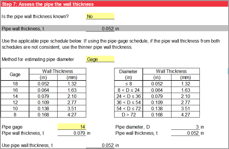
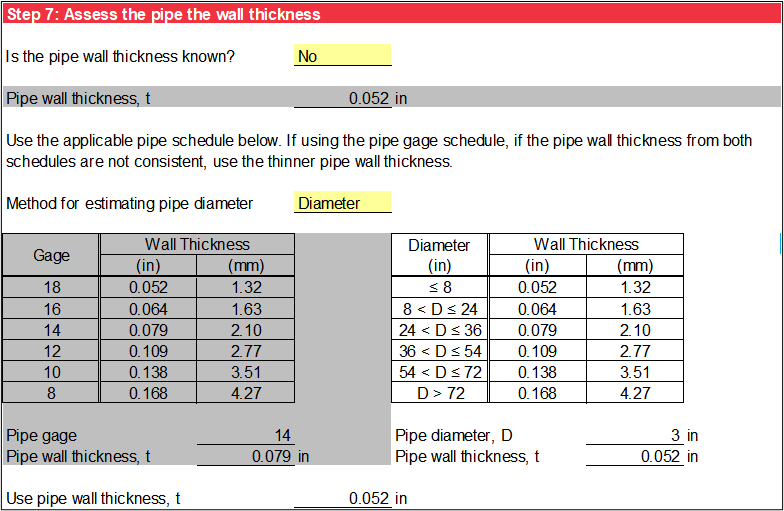
Step 7 assessed the pipe wall thickness. Commonly, plans only show the pipe gage and/or diameter. Using the drop-down list, select Yes if the pipe wall thickness is known, or No if the pipe wall thickness is unknown. For Yes, specify the pipe wall thickness as illustrated in Figure. For No, choose the method of estimating the pipe wall thickness using the drop-down list. The methods include Gage and Diameter. For Gage, choose the pipe gage, and the pipe wall thickness is estimated using a pipe gage and pipe schedule as illustrated in Figure. When using the pipe gage schedule, if the pipe wall thicknesses from both schedules are not consistent, use the thinner pipe wall thickness. For Diameter, specify the pipe diameter, and the pipe wall thickness is estimated using a pipe diameter schedule as illustrated in Figure. Cells that do not apply have a gray background.

Figure: Step 7 of Steel and Aluminum Pipe worksheet: User-specified pipe wall thickness.

Figure: Step 7 of Steel and Aluminum Pipe worksheet: Pipe wall thickness using pipe gage schedule.

Figure: Step 7 of Steel and Aluminum pipe worksheet: Pipe wall thickness using pipe diameter schedule.

Pipe Material Loss Rate

In step 8, the material loss rate (r_m) for steel and aluminum pipe is estimated based on the base metal type, flow likelihood, and deterioration environment as illustrated in Table and Table. The pipe material loss rates (inches per year) were developed by synthesizing several studies in a wide range of operating environments including, but not limited to, Ault and Ellor (2000) [?], Bednar (1989) [?], Bellair and Ewing (1984) [?], DeCou and Davies (2007) [?], Gabriel and Moran (1998) [?], Idaho Department of Highways (1965) [?], Jacobs (1982) [?], Kill (1969) [?], Malcom (1993) [?], Meacham (1982) [?], Missouri Highway and Transportation Department (1990) [?], Potter et al. (1991) [?], and Summerson and Hogan (1979) [?].

This step has no user-specified input. Cells that do not apply have a gray background.

Table: Material loss rate for traditional galvanized CSP and aluminum-zinc alloy-coated CSP (Galvalume® or equivalent).

Flow Likelihood	Material Loss Rate, rm (in/yr)
	Extremely Aggressive	Aggressive	Mild
Likely	0.0130	0.0028	0.00066
Unlikely	0.0055	0.0014	0.00036

Table: Material loss rate for aluminum-coated Type 2 CSP (ALCLAD® or equivalent).

Flow Velocity	Material Loss Rate, rm (in/yr)
	Extremely Aggressive	Aggressive	Mild
Likely	0.0178	0.00072	0.00019
Unlikely	0.0089	0.00036	0.00014

External Corrosion Protection System

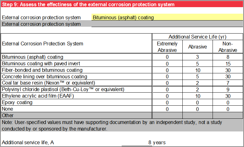
Step 9 assesses the effectiveness of the external corrosion protection system on the pipe. Select the type of external corrosion protection system using the drop-down list. Bituminous (asphalt) coating, bituminous coating with paved invert, fiber-bonded and bituminous coating, concrete-lined, coal tar base resin (Nexon^™ or equivalent), polyvinyl chloride plastisol (Beth-Cu-Loy^™ or equivalent), ethylene acrylic acid film, epoxy coating can be evaluated. Select None if no external corrosion protection system exists. The galvanized zinc coating that is typically applied to a CSP as part of the manufacturing process is not considered an external corrosion protection system.

The additional service life (A) is obtained from a table as a function of relative flow abrasiveness as illustrated in Figure. For extremely abrasive flow conditions, external corrosion protection systems are quickly worn away and do not provide additional years of service with respect to material loss rates (Potter et al. 1991) [?] and DeCou and Davies (2007) [?]. Similar to the evaluations of material loss rates for pipes, there are numerous studies investigating the effectiveness of external corrosion protection systems on drainage pipes. Studies by Bonds et al. (2005) [?], Potter et al. (1991) [?], Gabriel and Moran (1998) [?], and DeCou and Davies (2007) [?] were some of the evaluations used to develop the additional years of service life for external protection systems in this toolbox.

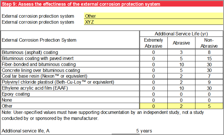
For Other, specify the additional service life as illustrated in Figure. Specified values must have supporting documentation by an independent study, not a study conducted by or sponsored by the manufacturer. The specified additional service life must be inversely proportional to the relative flow abrasiveness (as the relative abrasiveness increases, the additional service life must decrease).

Figure: Step 7 of Steel and Aluminum pipe worksheet: Pipe wall thickness using pipe diameter schedule.

Figure: Step 9 of Steel and Aluminum Pipe worksheet: User-specified additional service life.

Remaining Service Life

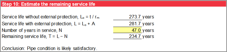
Step 10 calculates the remaining service life for the pipe as illustrated in Figure, both with and without external protection. The service life without external protection (L_o) is calculated by dividing the pipe wall thickness (t) by the material loss rate (r_m). The service life with external protection (L) is calculated by adding the additional service life due to the external protection system (A) to the service life without external protection (L_o).

Specify the number of years in service (N). The remaining service life (T) is calculated by subtracting the number of years of service (N) from the service life (L). If the remaining service life is less than or equal to 5 years, the cell has an orange background. A negative remaining service life is the number of years exceeding the service life.

If the remaining service life is greater than 5 years, the pipe condition is likely satisfactory. If the remaining service life is greater than or equal to -5 years and less than or equal to 5 years, the pipe is likely near the end of service life. If the remaining service life is less than -5 years, the pipe has likely exceeded service life.

Figure: Step 10 of Steel and Aluminum Pipe worksheet: Remaining service life.