Internal Erosion Suite

Sellmeijer

Between 1988 and 1993, Hans Sellmeijer and his coworkers developed a mathematical model for BEP progression. Curve-fitting numerical solutions in the process yielded a simplified calculation rule used in the Netherlands. The Sellmeijer model provided a relationship between pipe length and hydraulic head at which sand grains are in equilibrium. For any head less than the critical head (H_c), the development of the piping channels stops. If the head is increased, erosion begins again. The critical head occurs when the length of the channel (l) is about 0.3 to 0.5 of flow path length (L). For net hydraulic head (H) less than H_c, progression of the pipe reaches a stable condition. For H greater than H_c, the piping channel extends upstream and breaks through to the impounded water.

Sellmeijer’s model was implemented in a 2D numerical groundwater model to account for different configurations and used to derive a calculation rule for a standard levee located on top of a homogeneous confined aquifer. The original and adjusted calculation rules are described in Sellmeijer et al. (2011) [?]. The adjusted calculation rule extended and updated the piping model based on results of a wide range of tests (several small-scale, seven medium-scale, and four large-scale field Ijkdijk experiments). Thus, the Sellmeijer model is known to result in good predictions for large-scale experiments with 2D configurations. The method is applicable only within the limits of the piping model testing parameters shown in Table.

Table: Sellmeijer parameter limits.

Parameter	Minimum	Maximum
Particle size with 70 percent finer by weight, d70 (millimeters)	0.150	0.430
Coefficient of uniformity, U	1.3	2.6
Roundness of particles, KAS (percent)	35	70
Relative density, RD (percent)	50	100

Method of Analysis

The method of analysis is the same as the Schmertmann worksheet.

Soil Particle Characterization

Step 2 characterizes the soil particles in the piping layer. The input includes the specific gravity of sand particles (G_s), bedding angle of sand (θ), and White’s constant (η) as illustrated in Figure. The bedding angle and White’s constant are set to 37 degrees and 0.25, respectively, due to model calibration and are not changed in Dutch practice.

Figure: Step 2 of Sellmeijer worksheet: Discrete input.

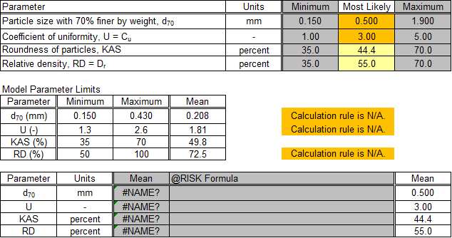
The selections in step 1 affect the remaining input for step 2. Cells that do not apply have a gray background. These cells are not used in subsequent calculations even if data is present. The input includes the particle size with 70 percent finer by weight (d₇₀), coefficient of uniformity (U), roundness of particles (KAS), and relative density (RD). The method is applicable only within the limits of the piping model testing parameters. Cells where the input parameter is outside the model parameter limits have an orange background, and a caution displays for those parameters. Mean values are used to normalize project-specific values.

The roundness of particles can be analyzed using optical images. Software such as ImageJ approximates an ellipse for each individual particle and calculates the roundness of each ellipse. For example, a perfect circle has a resulting roundness of 100 percent. Each image contains a variable number of particles, and multiple images of each soil sample should be analyzed. In practice, optical images of soil samples are rarely conducted to obtain KAS. Van Beek et al. (2009) [?] provides guidance for visual estimation of KAS as illustrated in Figure.

Figure: Step 2 of Sellmeijer worksheet: Visual estimate of KAS.

For deterministic analysis, input only the most likely values. The mean values used for subsequent calculations are the most likely (or mode) values. Figure illustrates the deterministic input.

Figure: Step 2 of Sellmeijer worksheet: Deterministic input.

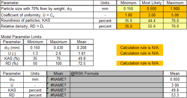
For probabilistic analysis without using @RISK, input the minimum and maximum values in addition to the most likely value, and triangular distributions represent the random variables. The mean values used in subsequent calculations are the average of the minimum, most likely, and maximum values. Figure illustrates the probabilistic input without using @RISK.

Figure: Step 2 of Sellmeijer worksheet: Probabilistic input without using @RISK.

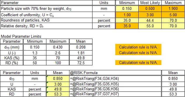
For probabilistic analysis using @RISK, input the minimum, most likely, and maximum values, and use an @RISK formula for a triangular distribution in the third column as a default. Alternatively, input a valid @RISK distribution in lieu of this default formula, and the user-specified input displays in the fourth column. The mean values used for subsequent calculations are the means for the @RISK distributions entered in the third column. Figure illustrates the probabilistic input using @RISK.

Figure: Step 2 of Sellmeijer worksheet: Probabilistic input using @RISK.

If using @RISK to perform probabilistic analysis, delete unnecessary calculation worksheets because the simulation is performed for all worksheets in the workbook, which this is time consuming. If cycling through iterations using @RISK, the displayed results are no longer mean values of the random variables; they are the selected iteration.

Piping Layer Characterization

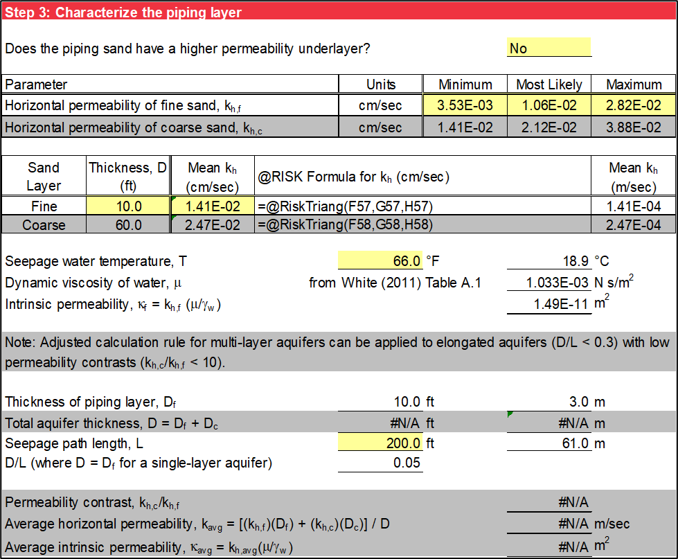
The selections in step 1 affect the input for step 3, and cells that do not apply have a gray background. These cells are not used in subsequent calculations even if data is present. Step 3 characterizes the piping layer. The input includes the horizontal permeability (k_h,f) and thickness (D_f) of the fine sand (piping) layer, seepage water temperature (T), and seepage path length (L). A lookup table is used to obtain the dynamic viscosity of water (μ) as a function of seepage water temperature.

The intrinsic permeability of the fine sand (piping) layer is calculated using Equation.

$$K_{f} = k_{h,f} \left(\frac{μ}{γ_w}\right)$$

where:

k_h = permeability of the fine sand (piping) layer in the horizontal direction (m/s)
μ = dynamic viscosity of water (N·s/m²)

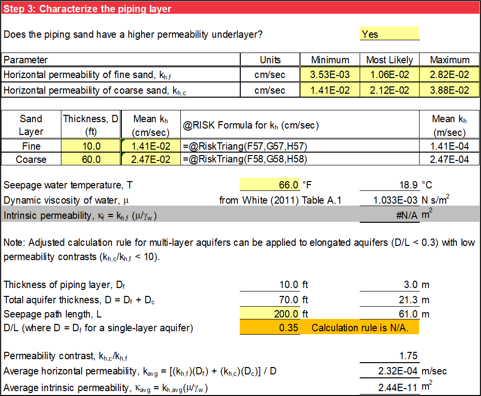
Use the drop-down list to indicate the presence of a multi-layer foundation (fine sand layer over coarse sand layer). Cells that do not apply have a gray background. Van Beek et al. (2012) [?] conducted piping experiments on multi-layer sand samples to validate Sellmeijer’s model, and the calculation rule was extended for multi-layer aquifers. A coarse layer beneath the piping layer increases the flow toward the pipe and decreases the critical head (and critical gradient). If a multi-layer foundation exists, the input also includes the horizontal permeability (k_h,c) and thickness (D_c) of the underlying coarse sand layer.

For a multi-layer aquifer, when flow toward the pipe is predominantly horizontal (for elongated aquifers), the increase of flow toward the pipe is reflected by the average horizontal permeability of a multilayer aquifer. A layer-weighted average of horizontal permeability (k_h,avg) is used in lieu of the horizontal permeability of the fine sand (piping) layer, shown in Figure, using Equation.

Figure: Step 3 of Sellmeijer worksheet: Multi-layer foundation input.

$$k_{h,avg} = \frac{k_{h,f}D_f + k_{h,c}D_{c}}{D}$$

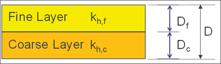
where:

k_h,f = permeability of the fine (piping) layer in the horizontal direction (centimeter/second)
D_f = thickness of the fine (piping) layer
k_h,c = permeability of the coarse underlayer in the horizontal direction (centimeter/second)
D_c = thickness of coarse underlayer (feet)
D = total aquifer thickness (feet)

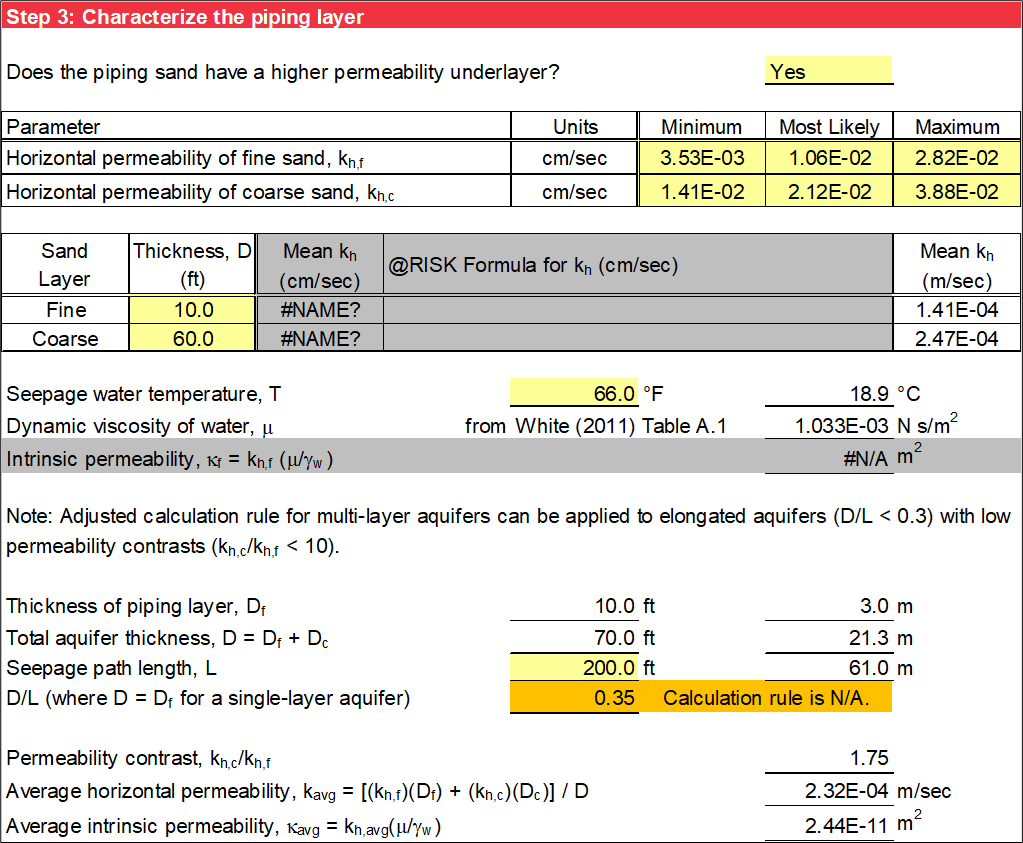
When the contrast of permeability is large and the aquifer thickness is relatively large compared to the seepage path length, assuming predominant horizontal flow is no longer valid. Hence, the extension of Sellmeijer’s calculation rule for multi-layer foundations can be applied to elongated aquifers $\left(\frac{D}{L}\right) < 0.3$ with low contrasts of permeability $\left(\frac{k_{h,c}}{k_{h,f}}\right) < 10)$. $\left(\frac{D}{L}\right)$ and $\left(\frac{k_{h,c}}{k_{h,f}}\right)$ values outside of these ranges have an orange background.

The average intrinsic permeability is calculated using Equation.

$$k_{avg} = k_{h,avg} \left(\frac{μ}{γ_w}\right)$$

For deterministic analysis of single-layer aquifer, input only the most likely value for the fine sand (piping) layer. The mean value used for subsequent calculations is the most likely (or mode) value. Figure illustrates the deterministic input for single-layer aquifer.

Figure: Step 3 of Sellmeijer worksheet: Deterministic input for single-layer aquifer.

For deterministic analysis of multi-layer aquifer, input the most likely values for the fine sand (piping) layer and underlying coarse sand layer. The mean values used for subsequent calculations are the most likely (or mode) values. Figure illustrates the deterministic input for multi-layer aquifer.

Figure: Step 3 of Sellmeijer worksheet: Deterministic input for multi-layer aquifer.

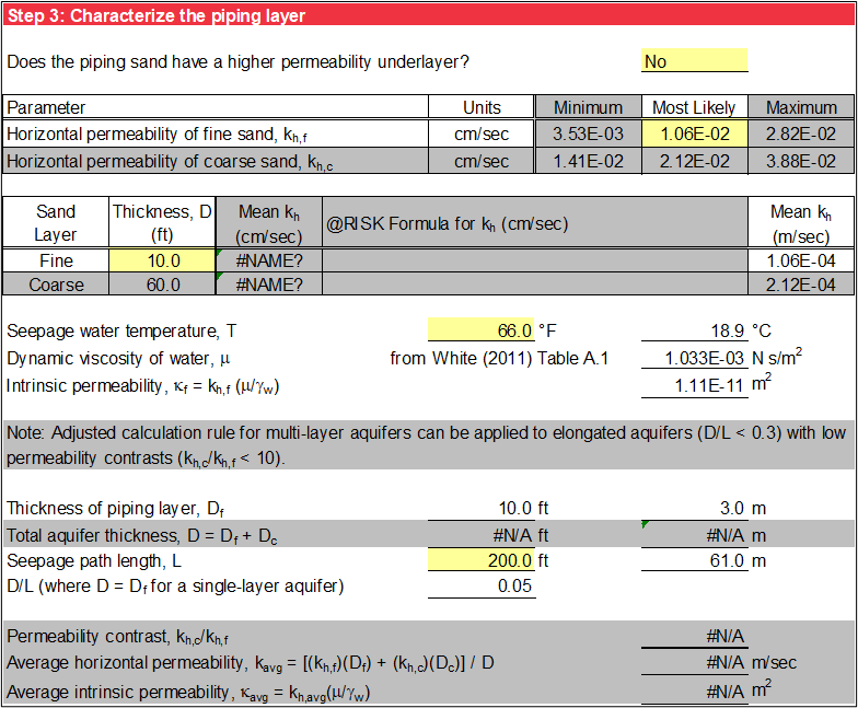
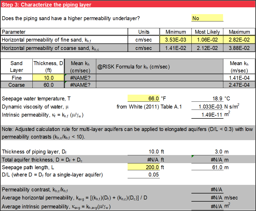
For probabilistic analysis of single-layer aquifer without using @RISK, input the minimum and maximum values in addition to the most likely value, and a triangular distribution represents the random variable for the fine sand (piping) layer. The mean value used in subsequent calculations is the average of the minimum, most likely, and maximum values. Figure illustrates the probabilistic input for single-layer aquifer without using @RISK.

Figure: Step 3 of Sellmeijer worksheet: Probabilistic input for single-layer aquifer without using @RISK.

For probabilistic analysis of multi-layer aquifer without using @RISK, input the most likely values for the fine sand (piping) layer and underlying coarse sand layer. The mean values used for subsequent calculations are the average of the minimum, most likely, and maximum values.

Figure illustrates the probabilistic input for multi-layer aquifer without using @RISK.

Figure: Step 3 of Sellmeijer worksheet: Probabilistic input for multi-layer aquifer without using @RISK.

For probabilistic analysis of single-layer aquifer using @RISK, input the minimum, most likely, and maximum values for the fine sand (piping) layer, and use an @RISK formula for a triangular distribution in the third column as a default. Alternatively, input a valid @RISK distribution in lieu of this default formula, and the user-specified input displays in the fourth column. The mean value used for subsequent calculations is the mean for the @RISK distribution entered in the third column. Figure illustrates the probabilistic input for single-layer aquifer using @RISK.

Figure: Step 3 of Sellmeijer worksheet: Probabilistic input for single-layer aquifer using @RISK.

For probabilistic analysis of multi-layer aquifer using @RISK, input the minimum, most likely, and maximum values for the fine sand (piping) layer and underlying coarse sand layer, and use an @RISK formula for a triangular distribution in the third column as a default. Alternatively, input a valid @RISK distribution in lieu of this default formula, and the user-specified input displays in the fourth column. The mean values used for subsequent calculations are the mean for the @RISK distribution entered in the third column. Figure the probabilistic input for multi-layer aquifer using @RISK.

Figure: Step 3 of Sellmeijer worksheet: Probabilistic input for multi-layer aquifer using @RISK.

Field Critical Horizontal Gradient for BEP Progression

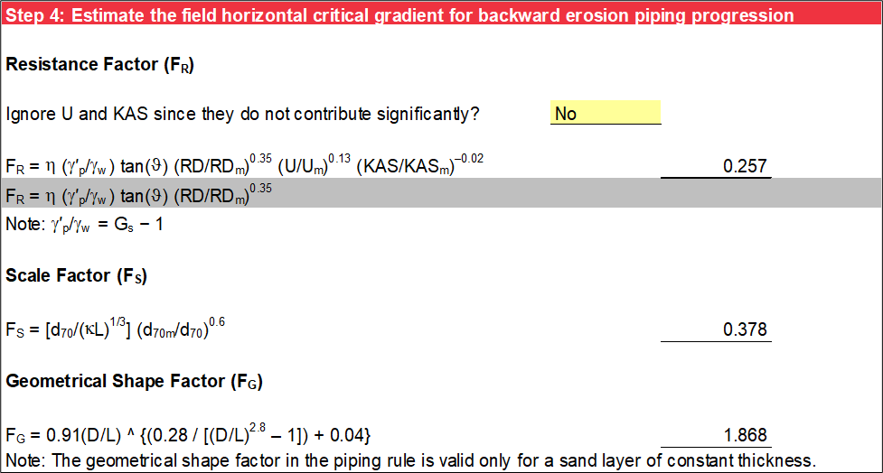
Step 4 calculates the field critical horizontal gradient for BEP progression as illustrated in Figure.

Equation, for the critical horizontal gradient for BEP progression (i_ch), is composed of three terms: a resistance factor that accounts for the strength of the layer subject to BEP; a scale factor that relates pore size and seepage size; and a geometrical shape factor.

$$i_{ch} = \left(F_R\right) \left(F_S\right) \left(F_G\right)$$

where:

F_R = resistance factor (strength of the layer subject to BEP)
F_S = scale factor (relating pore size and seepage size)
F_G = geometrical shape factor

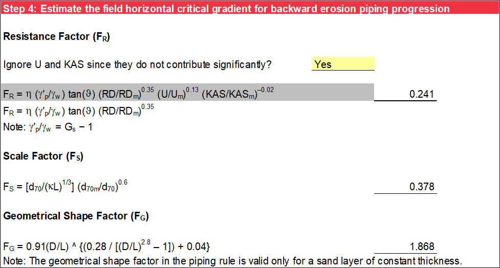
The resistance factor is a function of White's constant (η), bedding angle (θ), relative density (RD), roundness of the particles (KAS), and coefficient of uniformity (U) and is calculated using Equation.

$$F_R = η \left(\frac{γ'_p}{γ_w}\right) \tanθ \left(\frac{RD}{72.5}\right)^{0.35} \left(\frac{U}{1.81}\right)^{0.13} \left(\frac{KAS}{49.2}\right)^{-0.02}$$

where:

KAS = roundness of the particles (percent)
RD = relative density (percent)
U = coefficient of uniformity
γ'_p = submerged unit weight of soil particles (N/m³)
γ_w = unit weight of water (N/m³)
θ = bedding angle (degrees)
η = White's constant

Since it is easier to estimate the specific gravity of soil particles than the submerged unit weight of soil particles, the substitution in Equation is made to the equation for F_R.

$$\frac{γ'_p}{γ_w} = G_s - 1$$

The bedding angle and White’s constant have been set to 37 degrees and 0.25, respectively, due to model calibration and are not changed in Dutch practice. Since the values were fixed in the multi-variate regression, any influence they had is accounted for in related variables. It is, therefore, not appropriate to vary these parameters.

Van Beek et al. (2010) [?] indicate that KAS and U appear less important than other sand characteristics, and the results of multivariate regression analysis show that they have a weak influence on critical gradient. Therefore, U and KAS terms in equation for F_R are sometimes ignored in practice. The toolbox provides an option to neglect the expressions containing these terms from the equation for F_R as illustrated in Figure.

The scale factor is a function of the particle size for which 70 percent is finer (by weight) (d₇₀), the horizontal seepage path length (L), and the intrinsic permeability of the piping layer (κ) and is calculated using Equation.

$$F_S = \left(\frac{d_{70}}{κL}\right)^{\frac{1}{3}} \left(\frac{0.000208}{d_{70}}\right)^{0.6}$$

where:

d₇₀ = particle size (m) for which 70 percent is finer (by weight)
κ = intrinsic permeability (m²) of the piping layer

The intrinsic permeability of the piping layer in Equation 20 is either κ_f for a single-layer aquifer or k_h,avg for a multi-layer aquifer.

The value of the horizontal permeability used to calculate the intrinsic permeability depends on the selection in step 3. For single-layer aquifers, it is the value for the fine sand (piping) layer. For multi-layer aquifers, it is the layer-weighted average.

The geometrical factor is a function of the ratio of the depth of the piping layer to the horizontal seepage path length $\left(\frac{D}{L}\right)$ and is calculated using Equation.

$$F_G = 0.91 \left(\frac{D}{L}\right)^{\frac{0.28}{\left(\frac{D}{L}\right)^{2.8} - 1} + 0.04}$$

where:

D = thickness of the piping layer (m) where D = D_f for a single-layer aquifer
L = seepage path length (m) through the piping layer (measured horizontally)

Figure: Step 4 of Sellmeijer worksheet: Critical gradient terms with U and KAS.

Figure: Step 4 of Sellmeijer worksheet: Critical gradient terms without U and KAS.

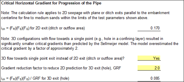
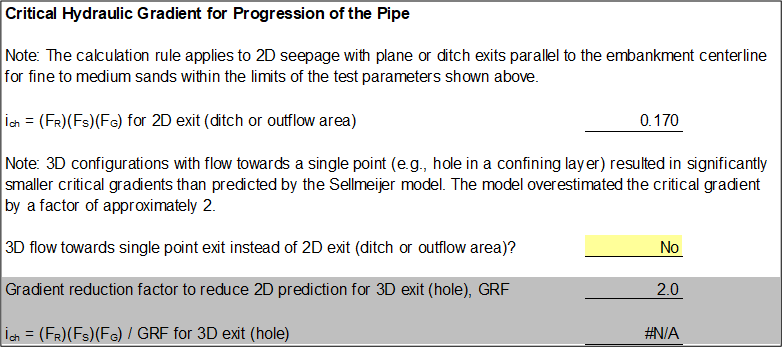
Sellmeijer’s model applies to 2D seepage with plane or ditch exits parallel to the embankment centerline for fine to medium sands within the limits of the model test parameters. Van Beek et al. (2015) [?] found that 3D configurations with flow toward a single point (such as a hole in a confining layer) resulted in significantly smaller critical gradients than predicted by the adjusted calculation model. In both the small and medium-scale experiments, the model overestimated the critical gradient by a factor of approximately two. If the field horizontal critical gradient is further adjusted for 3D flow, input a user-specified GRF. Cells that do not apply have a gray background. The two scenarios are illustrated in Figure and Figure.

Figure: Step 4 of Sellmeijer worksheet: Field critical gradient with gradient reduction factor.

Figure: Step 4 of Sellmeijer worksheet: Field critical gradient without gradient reduction factor.

Likelihood of Backward Erosion Piping Progression

Step 5 calculates the average hydraulic gradient in the foundation by dividing the net hydraulic head by the seepage path length using Equation.

$$i_{avf} = \frac{\Delta H}{L} = \frac{HW - TW}{L}$$

where:

∆H = net hydraulic head (feet)
HW = headwater level (feet)
TW = tailwater level (feet)
L = seepage path length (feet)

The FS against BEP progression is calculated using Equation.

$$FS = \frac{i_{ch}}{i_{avf}}$$

where:

i_ch = critical horizontal gradient for BEP progression
i_avf = average horizontal gradient in the foundation at the pipe head

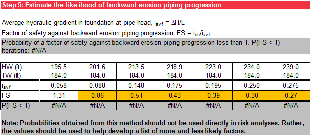
For deterministic analysis, the FS is calculated using the most likely values of the random variables and is summarized in a table. Cells that do not apply have a gray background.

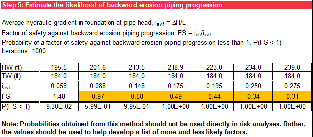
For probabilistic analysis, the FS is calculated as described for the deterministic analysis but for the mean values of the random variables, and multiple iterations are performed by sampling the distributions in step 2. The probability of BEP progression is equal to the percentage of iterations that resulted in an FS less than 1 [P(FS < 1)].

For probabilistic analysis performed without using @RISK, 1,000 iterations are used. For probabilistic analysis using @RISK, the number of iterations is user-specified, and “@RISK” displays in parentheses after the number of iterations for this scenario. If cycling through iterations using @RISK, the displayed results are no longer mean values; they are the selected iteration’s values.

For deterministic and probabilistic analyses, cells with FS less than 1 have an orange background. Figure illustrates the deterministic tabular output, and Figure illustrates the probabilistic tabular output without using @RISK.

Figure: Step 5 of Sellmeijer worksheet: Deterministic tabular output.

Figure: Step 5 of Sellmeijer worksheet: Probabilistic tabular output without using @RISK.

Summary Plots

Step 6 generates the summary plots. The first plot is the mean FS against BEP progression (red solid line) and average horizontal gradient at the pipe head (green solid line) as functions of headwater level. If cycling through iterations using @RISK, the displayed results are no longer mean values; they are the selected iteration. FS against BEP progression is plotted on the primary axis, and average horizontal gradient at the pipe head is plotted on the secondary axis. Horizontal reference lines display for the mean field critical gradient for BEP progression (green dashed line) and FS of 1 (red shaded line). Figure illustrates the deterministic graphical output.

Figure: Step 6 of Sellmeijer worksheet: Deterministic graphical output.

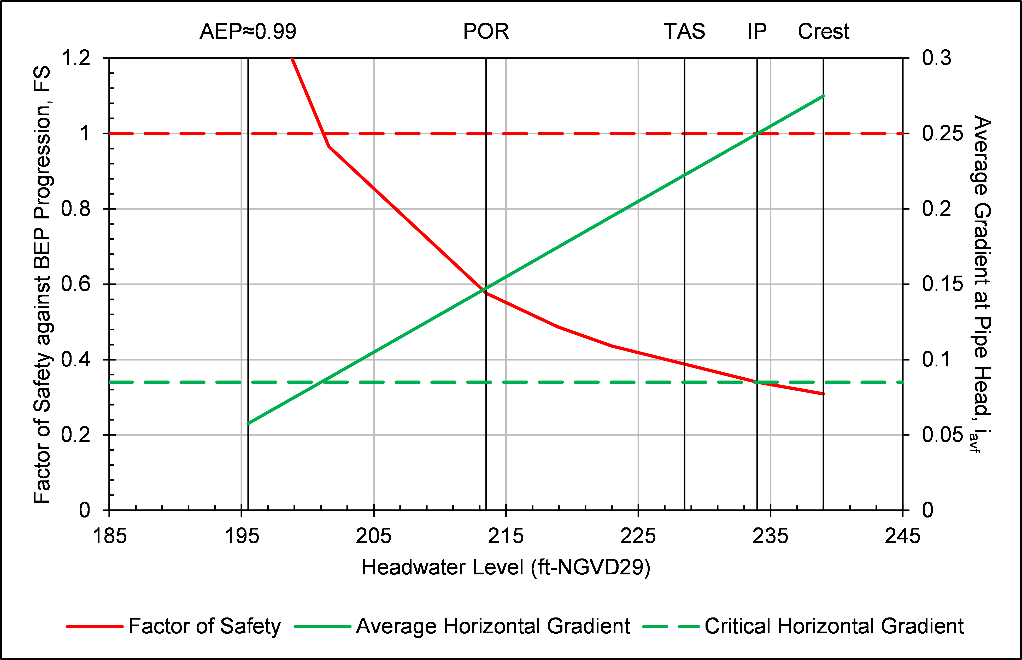
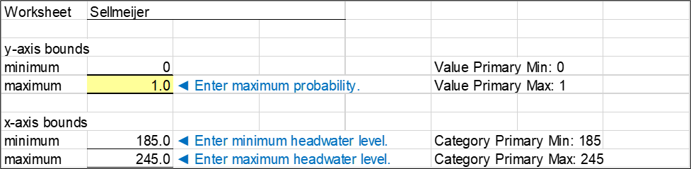
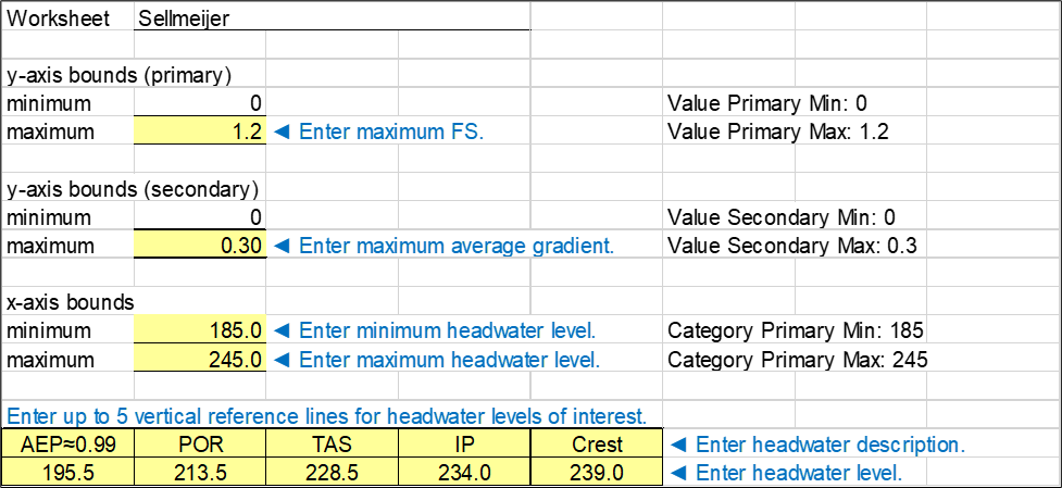
Figure illustrates the plot options for this chart. The maximum value for the primary y-axis (FS against BEP progression), maximum value for the secondary y-axis (average horizontal gradient at the pipe head), and minimum and maximum values for the x-axis (headwater level) are user-specified. Users can input up to five vertical reference elevations, and user-specified labels display at the top of the chart.

Figure: Step 6 of Sellmeijer worksheet: Plot options for deterministic graphical output.

For probabilistic analysis, the mean probability of BEP progression is plotted as a function headwater level. If cycling through iterations using @RISK, this plot has a gray background because the probability of initiation cannot be calculated from a single iteration. Similarly, this plot has a gray background for deterministic analysis. Figure illustrates the graphical output for probabilistic analysis.

Figure: Step 6 of Sellmeijer worksheet: Probabilistic graphical output.

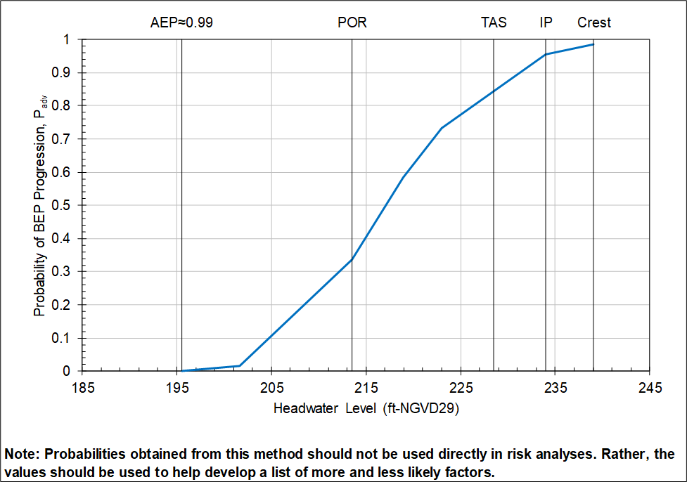
Figure illustrates the plot options for this chart. The vertical reference elevations and minimum and maximum values for the x-axis (headwater level) are the same as the input for the previous chart. Only the maximum value for the y-axis (probability of BEP progression) is user-specified.

Figure: Step 6 of Sellmeijer worksheet: Plot options for probabilistic graphical output.