Internal Erosion Suite

Schmertmann

Schmertmann (2000) [?] developed an approach for estimating the factor of safety (FS) regarding piping using the concept of ambient, pre-pipe, hydraulic gradients along the potential piping path based on laboratory flume tests. The FS for pipe progression is given in Equation:

$$FS = \left(\frac{C_D C_L C_S C_K C_γ C_Z C_α i_{\textit{pmt}}}{C_R i_f}\right)$$

where:

i_pmt = maximum pre-pipe hydraulic gradient along the pipe path in the reference laboratory test (that is, laboratory horizontal critical gradient)
i_f = maximum pre-pipe hydraulic gradient along the pipe path in the field
C_D = depth/length factor
C_L = total pipe length factor
C_S = grain-size factor
C_K = anisotropic permeability factor
C_γ = density factor
C_Z = underlayer factor
C_α = adjustment for pipe inclination
C_R = embankment axis curvature factor

Schmertmann applied these correction factors to more than 100 laboratory flume tests to adjust the laboratory results to the reference values shown in Table.

Table: Schmertmann reference test values

Parameter	Minimum
Seepage path length, L	5 feet
Piping Layer Depth, D	1 foot
Particle size with 10% passing by weight, d10	0.20 millimeters
Anisotropy, $R_k = \frac{k_h}{k_v}$	1.5
Relative density, Dr	60 percent
Pipe path inclination, α	0 degrees

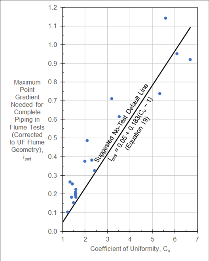
From the corrected values, Schmertmann proposed a no-test default relationship as the default value of i_pmt to use in assessments if laboratory flume tests were not conducted, shown in Equation and Figure.

$$i_{pmt} = 0.05 + 0.183(C_u - 1)$$

where

C_u = coefficient of uniformity

Figure: Schmertmann laboratory critical gradients.

Equation and Equation can be used along with the correction factors to assess the FS for BEP progression in the field. While this figure is quite useful, it is difficult to estimate the uncertainty in the critical point gradient because study averages were presented. For example, one of the single data points is the average from 14 individual laboratory tests.

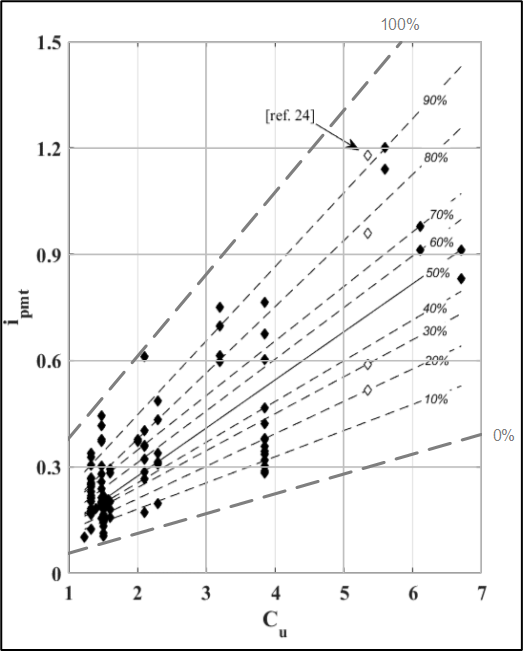
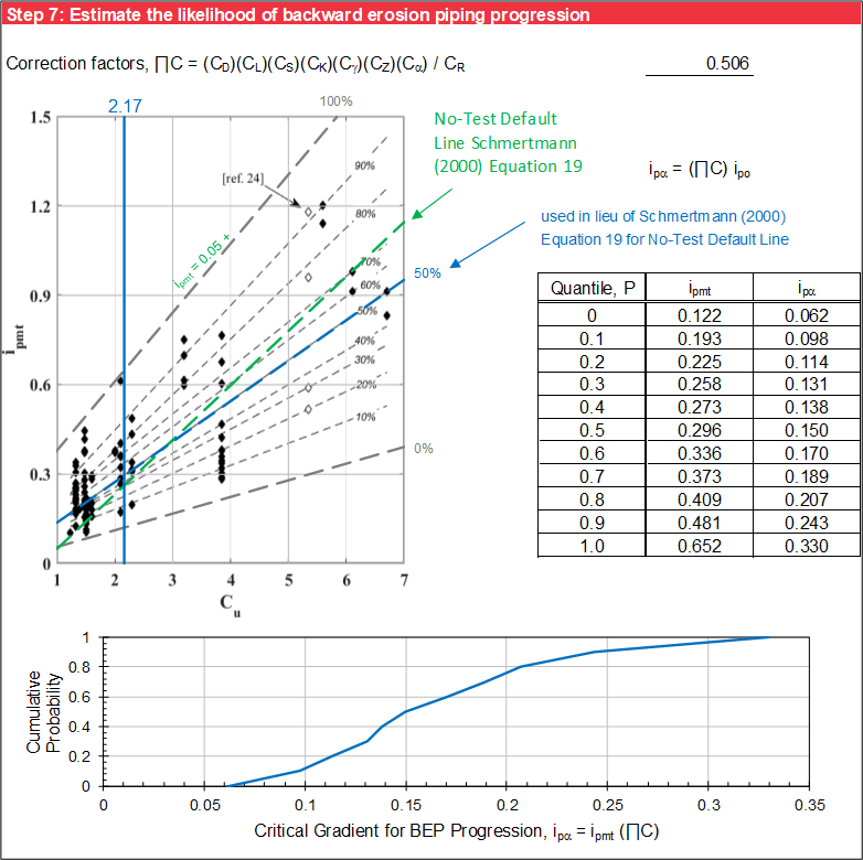
To assess the likelihood of BEP progression, Robbins and Sharp (2016) [?] compiled all the data in Schmertmann (2000) [?] and developed a probabilistic chart for determining ipmt, again relative to the reference values, as shown in Figure. Robbins and O’Leary (2020) [?] expanded this chart to include 0 percent and 100 percent probability trend lines based on linear extrapolation of the slopes and intercepts of the quantile regression lines.

Figure: Schmertmann laboratory critical gradients with Robbins and Sharp (2016) estimated probability curves and Robbins and O’Leary (2020) modifications.

To calculate a probability of BEP progression using the lines shown on the probability chart, the value of i_pmt must be calculated for a given field scenario as shown in Equation.

$$i_{pmt} = \frac{{C_R}{i_f}} {{C_D}{C_L}{C_S}{C_K}{C_γ}{C_Z}{C_α}}$$

The probabilistic chart from Robbins and Sharp (2016) [?] shows that the uncertainty with the laboratory critical gradient increases with increasing C_u, where there is less data. In addition, at higher C_u values, soils tend to become internally unstable. Therefore, the probabilistic chart is limited to a C_u between 1.1 and about 4.

Method of Analysis

In step 1, use the drop-down list to select the method of analysis (probabilistic or deterministic). There are two options for probabilistic analysis. The first performs 1,000 iterations (judged adequate for most applications) without using Palisade's @RISK software. This provides flexibility if an @RISK software license is not available. The second uses @RISK to customize the probabilistic analysis. Use the drop-down list to select Yes if @RISK is to be used and No if @RISK is not used. The three possible scenarios are illustrated in Figure through Figure.

Figure: Step 1 of Schmertmann worksheet: Deterministic analysis.

Figure: Step 1 of Schmertmann worksheet: Probabilistic analysis without using @RISK.

Figure: Step 1 of Schmertmann worksheet: Probabilistic analysis using @RISK.

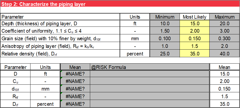
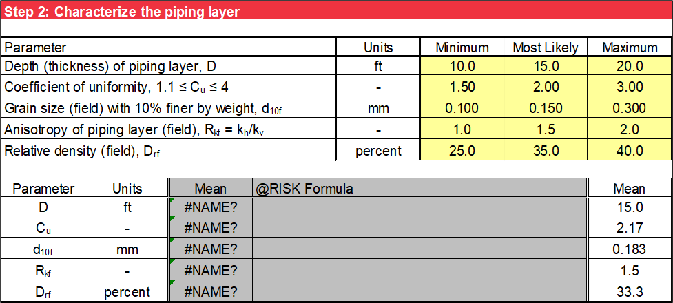
Piping Layer Characterization

Step 2 characterizes the piping layer. The input includes the depth (thickness) of the piping layer (D), coefficient of uniformity (C_u), grain size in the field with 10 percent finer by weight (d_10f), anisotropy in the field of the piping layer (R_kf), relative density in the field (D_rf), and angle of the pipe path (α). The adjusted Schmertmann method uses the probabilistic chart of Robbins and Sharp (2016) [?], expanded by Robbins and O’Leary (2020) [?], for both the deterministic and probabilistic methods and is limited to C_u between 1.1 and 4. C_u values outside of this range have an orange background. The depth (thickness of the piping layer) is in the direction perpendicular to the angle of the pipe path discussed later in this section.

The selections in Step 1 affect the input for Step 2, and cells that do not apply have a gray background. These cells are not used in subsequent calculations even if data is present.

For deterministic analysis, input only the most likely values. The mean value used for subsequent calculations is the most likely (or mode) value. Figure illustrates the deterministic input.

Figure: Step 2 of Schmertmann worksheet: Deterministic input.

For probabilistic analysis without using @RISK, input the minimum and maximum values in addition to the most likely value, and triangular distributions represent the random variables. The mean values used in subsequent calculations are the average of the minimum, most likely, and maximum values. Figure illustrates probabilistic input without using @RISK.

Figure: Step 2 of Schmertmann worksheet: Probabilistic input without using @RISK.

For probabilistic analysis using @RISK, input the minimum, most likely, and maximum values, and use an @RISK formula for a triangular distribution in the third column as a default. Alternatively, input a valid @RISK distribution in lieu of this default formula, and the user-specified input displays in the fourth column. The mean values used for subsequent calculations are the means for the @RISK distributions entered in the third column. Figure illustrates the probabilistic input without using @RISK.

Figure: Step 2 of Schmertmann worksheet: Probabilistic input using @RISK.

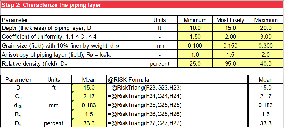
If using @RISK to perform probabilistic analysis, delete unnecessary calculation worksheets because the simulation is performed for all worksheets in the workbook, which is time consuming. If cycling through iterations using @RISK, the displayed results are no longer mean values of the random variables; they are the selected iteration’s values.

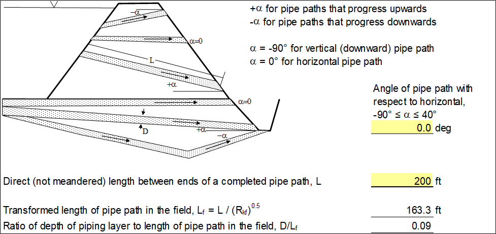
The remaining input for step 2 addresses pipe path geometry as illustrated in Figure and includes the angle of the pipe path (α) with respect to horizontal and the direct (not meandered) length between ends of a completed pipe path (L). A figure is included in this step as a guide.

In most cases, the pipe path is horizontal, and α = 0 degrees. The angle is positive for pipe paths that progress upwards and negative for pipe paths that progress downwards. Based on Schmertmann (2000) [?], the range for α is between -90 degrees and 40 degrees. Cells where the input parameter is outside these limits have an orange background.

Based on the user-specified anisotropy, the ratio of the depth of the piping layer to the length of the pipe path in the field $\left(\frac{D}{L_f}\right)$ is calculated, and the transformed length of the piping path in the field (L_f) is calculated using Equation.

$$L_f = \frac{L} {(R_{kf})^{0.5}}$$

where:

R_kf = anisotropy in the field of the piping layer (k_h/k_v)

Figure: Step 2 of Schmertmann worksheet: Pipe path geometry.

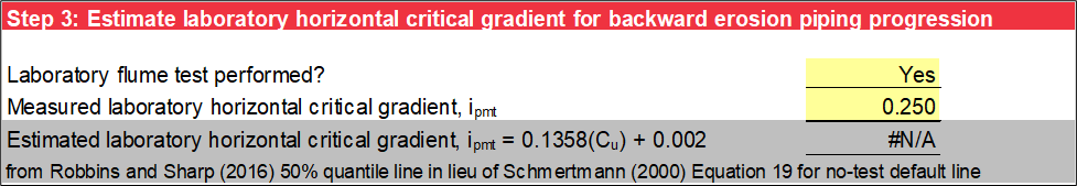
Laboratory Horizontal Critical gradient

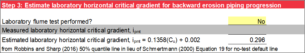
Step 3 estimates the laboratory horizontal critical gradient. Use the drop-down list to indicate if a laboratory flume test was performed. Cells that do not apply have a gray background. For a laboratory flume test, input the measured laboratory horizontal critical gradient as illustrated in Figure. In practice, laboratory flume tests are rarely conducted to measure the critical horizontal gradient, and the linear relationship proposed by Schmertmann (2000) [?] is the primary means for estimating critical gradient values as a function of coefficient of uniformity (C_u). In this toolbox, the 50 percent quantile line from Robbins and Sharp (2016) [?] is used in lieu of Schmertmann’s no-test default line using Equation as illustrated in Figure.

$$i_{pmt} = 0.1358(C_u) + 0.002$$

Robbins and Sharp found that the best fit, median line of all test results indicates Schmertmann's no-test default line is conservative for C_u < 3 and unconservative for C_u > 3.

Figure: Step 3 of Schmertmann worksheet: Critical gradient from laboratory flume test.

Figure: Step 3 of Schmertmann worksheet: Estimated laboratory critical gradient.

Field Horizontal Critical Gradient

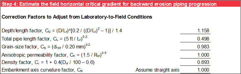
Step 4 calculates the field horizontal critical gradient by applying the various correction factors to the estimated or measured laboratory horizontal critical gradient as illustrated in Figure. The correction factors for foundation depth, seepage path length, grain size, anisotropy, and soil density are estimated using Equation, Equation, Equation, Equation, and Equation. Since a straight axis is assumed for the embankment, there is no correction factor for curvature in the embankment axis, and C_R = 1.

$$C_D = \frac{\left(\frac{D}{L_f}\right)^{\frac{0.2}{\left(\frac{D}{L_f}\right)^2-1}}}{\left(\frac{1 ft}{5 ft}\right)^{\frac{0.2}{\left(\frac{1 ft}{5 ft}\right)^2-1}}} = \frac{\left(\frac{D}{L_f}\right)^{\frac{0.2}{\left(\frac{D}{L_f}\right)^2-1}}}{1.4}$$

$$C_L = \left(\frac{5 ft}{L_f}\right)^{0.2}$$

$$C_S = \left(\frac{d_{10f}}{0.20 mm}\right)^{0.2}$$

$$C_K = \left(\frac{1.5}{\frac{k_h}{k_v}}\right)^{0.5} = \left(\frac{1.5}{R_{kf}}\right)^{0.5}$$

$$C_γ = 1 + 0.4\left(\frac{D_{rf}}{100}-0.6\right)$$

where:

$\frac{D}{L_f}$ = ratio of depth of piping layer to length of pipe path in the field
L_f = transformed length (feet) of the pipe path in the field
$\frac{k_h}{k_v}$ = anisotropy in the field (R_kf)
D_rf = relative density in the field

Figure: Step 4 of Schmertmann worksheet: Corrections for field conditions.

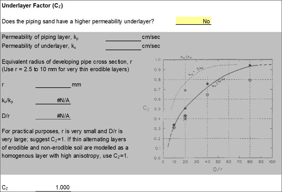
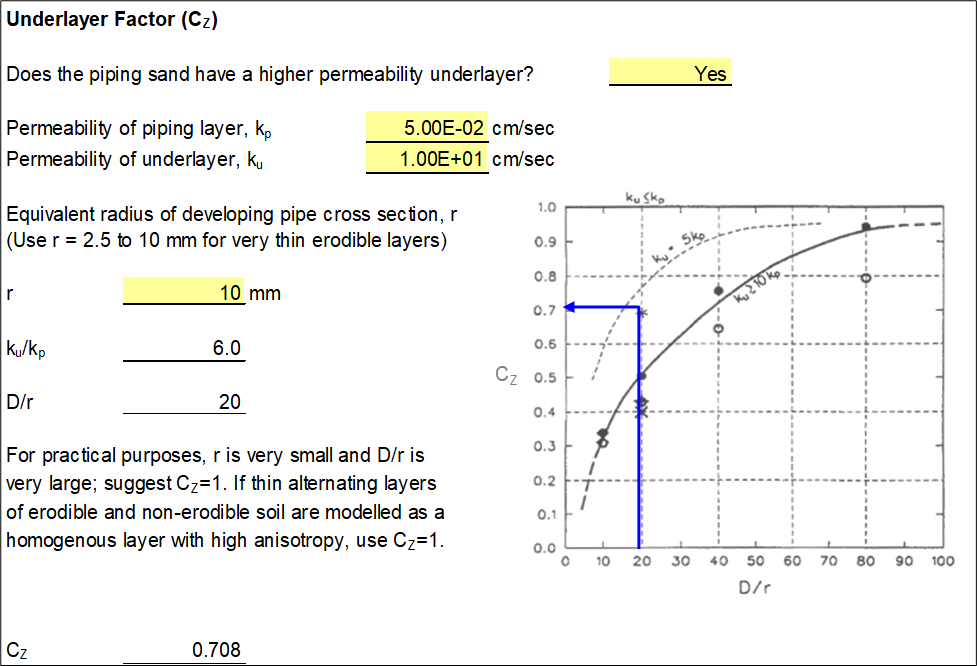
A higher permeability layer beneath the piping layer increases the flow toward the pipe and decreases the critical gradient. Use the drop-down list to indicate the presence of a higher permeability underlayer (for example, fine sand layer over coarse sand layer). If there is no higher permeability underlayer, C_Z = 1 as illustrated in Figure. Cells that do not apply have a gray background. If a higher permeability underlayer exists, input the permeability of the piping layer (k_p), permeability of the underlayer (k_u), and equivalent radius of the developing pipe cross section (r) to estimate the underlayer correction factor (C_Z).

Schmertmann (2000) [?] provided C_Z as a function of $\left(\frac{D}{r}\right)$ for $\left(\frac{k_u}{k_p}\right) ≤ 1$, $\left(\frac{k_u}{k_p}\right) = 5$, and $\left(\frac{k_u}{k_p}\right) ≥ 1$ based on very limited data derived from flow nets of the University of Florida flume. C_Z is obtained from two-way linear interpolation using these three curves as illustrated in Figure. Fell et al. (2008) [?] suggests using C_Z = 1 since r is very small and $\left(\frac{D}{r}\right)$ is typically very large in practice; C_Z is approximately 1 when $\left(\frac{D}{r}\right)$ is greater than about 80. For very thin erodible layers (less than a couple of feet), Fell et al. (2008) [?] suggested using r = 2.5 to 10 mm, where the horizontal critical gradient decreases as r increases. If thin alternating layers of erodible and non-erodible soil are modeled as a homogenous layer with high anisotropy, use C_Z = 1.

Figure: Step 4 of Schmertmann worksheet: No underlayer factor.

Figure: Step 4 of Schmertmann worksheet: Underlayer factor.

The field horizontal critical gradient is calculated using the above correction factors and Equation as illustrated in Figure.

$$i_{ch} = \left(\frac{C_D C_L C_S C_K C_γ C_Z}{C_R}\right)i_{pmt}$$

Figure: Step 4 of Schmertmann worksheet: Field horizontal critical gradient.

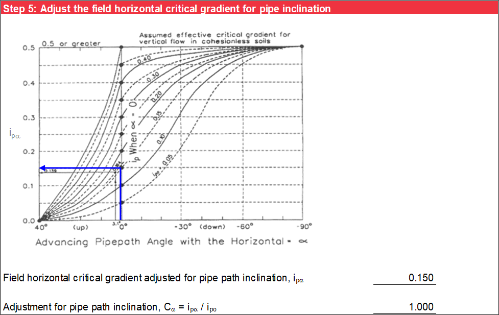
Pipe Path Inclination

Step 5 determines the adjustment for pipe path inclination. In most cases, the pipe path is horizontal (α = 0 degrees), and C_α= 1. Cells that do not apply have a gray background. If the pipe path inclination is not zero, Schmertmann (2000) [?] provided the field critical gradient adjusted for pipe path inclination (i_pα) as a function of α for field horizontal critical gradients (i_po) of 0.05, 0.10, 0.15, 0.20, 0.25, 0.30, 0.35, 0.40, 0.45, and 0.50 or greater, as illustrated in Figure. i_pα is obtained from two-way linear interpolation using these ten curves. The back-calculated adjustment for pipe path inclination uses Equation.

$$C_α = \frac{i_{pα}}{i_{po}}$$

Figure: Step 5 of Schmertmann worksheet: Adjustment for pipe path inclination.

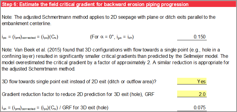
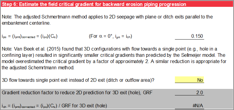
Field Critical Gradient for BEP progression

Step 6 adjusts the field horizontal critical gradient for pipe path inclination using the adjustment for pipe path inclination (C_α) from step 4 using Equation.

$$i_{pα} = i_{ch} C_α$$

If the pipe path is horizontal, i_pα = i_ch because C_α = 1.

Schmertmann’s adjusted model applies to 2D seepage with plane or ditch exits parallel to the embankment centerline. Van Beek et al. (2015) [?] found that three-dimensional (3D) configurations with flow toward a single point (such as a hole in a confining layer) resulted in significantly smaller critical gradients than predicted by the Dutch piping model. In both the small and medium-scale experiments, the model overestimated the critical gradient by a factor of approximately two. Although not developed and calibrated for this method, a similar reduction for a 3D exit condition is appropriate. If the field horizontal critical gradient is further adjusted for 3D flow, input a user-specified gradient reduction factor (GRF). Cells that do not apply have a gray background. Figure and Figure illustrate the two scenarios.

Figure: Step 6 of Schmertmann worksheet: Field critical gradient with gradient reduction factor.

Figure: Step 6 of Schmertmann worksheet: Field critical gradient without gradient reduction factor.

Likelihood of Backward Erosion Piping Progression

Robbins and Sharp (2016) [?] presented the results of a best-fit quantile regression analysis from the individual laboratory flume tests, which were expanded by Robbins and O'Leary (2020) [?] to include 0 percent and 100 percent probability trend lines based on linear extrapolation of the slopes and intercepts of the quantile regression lines. Step 7 uses this modified chart to develop a cumulative density function to estimate the probability of BEP progression as illustrated in Figure.

Figure: Step 7 of Schmertmann worksheet: Cumulative density function for backward erosion piping progression.

The average horizontal gradient in the foundation at the pipe head is calculated by dividing the net hydraulic head by the seepage path length using Equation.

$$i_{avf} = \frac{ΔH}{L} = \frac{HW-TW}{L}$$

where:

ΔH = net hydraulic head (feet)
HW = headwater level (feet)
TW = tailwater level (feet)
L = direct (not meandered) seepage path length (feet)

The FS against BEP progression is calculated using Equation.

$$FS = \frac{i_{pα}}{i_{avf}}$$

where:

i_pα = critical gradient for BEP progression (adjusted for pipe path inclination)
i_avf = average horizontal gradient in the foundation at the pipe head

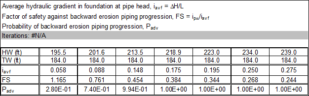
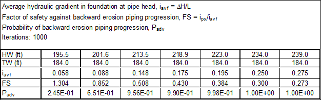
For deterministic analysis, the FS is calculated using the most likely values of the random variables and summarized in a table. Cells that do not apply have a gray background. For probabilistic analysis, the FS is calculated as described for the deterministic analysis but for the mean values of the random variables, and multiple iterations are performed by sampling the distributions in step 2. The probability of BEP progression is equal to the percentage of iterations that resulted in a FS less than 1 [P(FS < 1)]. For probabilistic analysis performed without using @RISK, 1,000 iterations are used. For probabilistic analysis using @RISK, the number of iterations is user-specified, and “@RISK” displays in parentheses after the number of iterations for this scenario. If cycling through iterations using @RISK, the displayed results are no longer mean values; they are the selected iteration’s values. For deterministic and probabilistic analyses, cells with FS less than 1 have an orange background. Figure illustrates the deterministic tabular output, and Figure illustrates the probabilistic tabular output without using @RISK.

Figure: Step 7 of Schmertmann worksheet: Tabular output for deterministic analysis.

Figure: Step 7 of Schmertmann worksheet: Tabular output for probabilistic analysis without using @RISK.

Summary Plots

Step 8 generates the summary plots. The first plot is the mean FS against BEP progression (red solid line) and average horizontal gradient at the pipe head (green solid line) as functions of headwater level. If cycling through iterations using @RISK, the displayed results are no longer mean values; they are the selected iteration. FS against BEP progression is plotted on the primary axis, and average horizontal gradient at the pipe head is plotted on the secondary axis. Horizontal reference lines display for the mean field critical gradient for BEP progression (green dashed line) and FS of 1 (red shaded line).

Figure illustrates the deterministic graphical output.

Figure: Step 7 of Schmertmann worksheet: Graphical output for deterministic analysis.

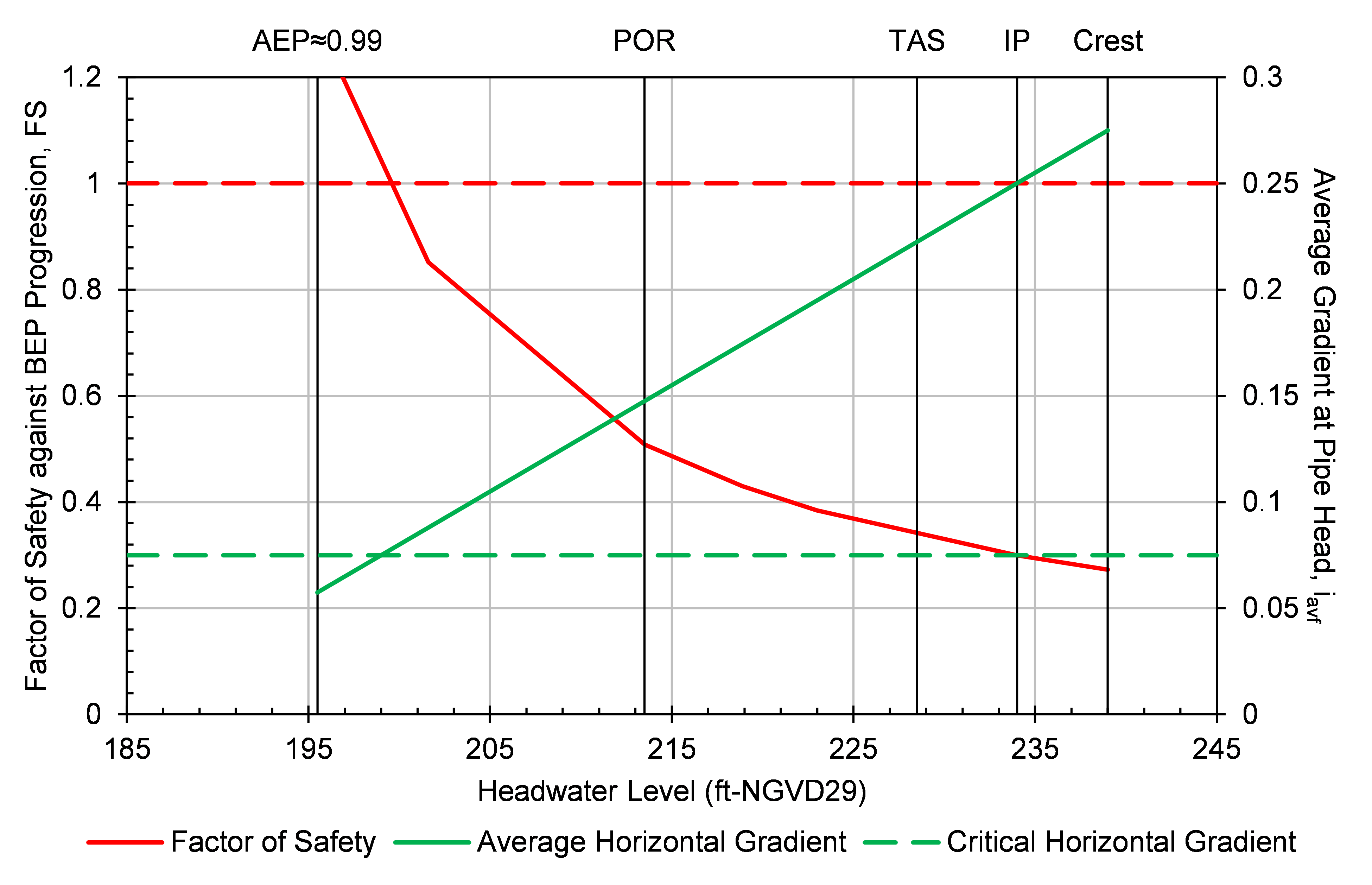
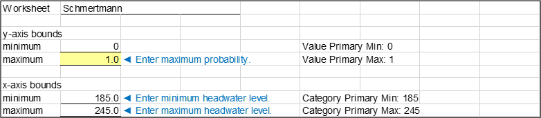
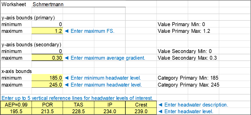
Figure illustrates the plot options this chart. The maximum value for the primary y-axis (FS against BEP progression), maximum value for the secondary y-axis (average horizontal gradient at the pipe head), and minimum and maximum values for the x-axis (headwater level) are user-specified. Users can input up to five vertical reference elevations, and user-specified labels display at the top of the chart.

Figure: Step 7 of Schmertmann worksheet: Plot options for deterministic analysis.

Because the adjusted Schmertmann method uses the probabilistic chart of Robbins and Sharp (2016) [?], expanded by Robbins and O’Leary (2020) [?], a probability of BEP progression is calculated for both the deterministic and probabilistic methods as illustrated in Figure and Figure, respectively. The mean probability of BEP progression is plotted as a function headwater level. For probabilistic analysis, the 90 percent uncertainty bounds (5th and 95th percentiles) are also plotted as a function headwater level using dashed lines, as shown in Figure.

Figure: Step 7 of Schmertmann worksheet: Graphical output for deterministic analysis.

Figure: Step 7 of Schmertmann worksheet: Graphical output for probabilistic analysis.

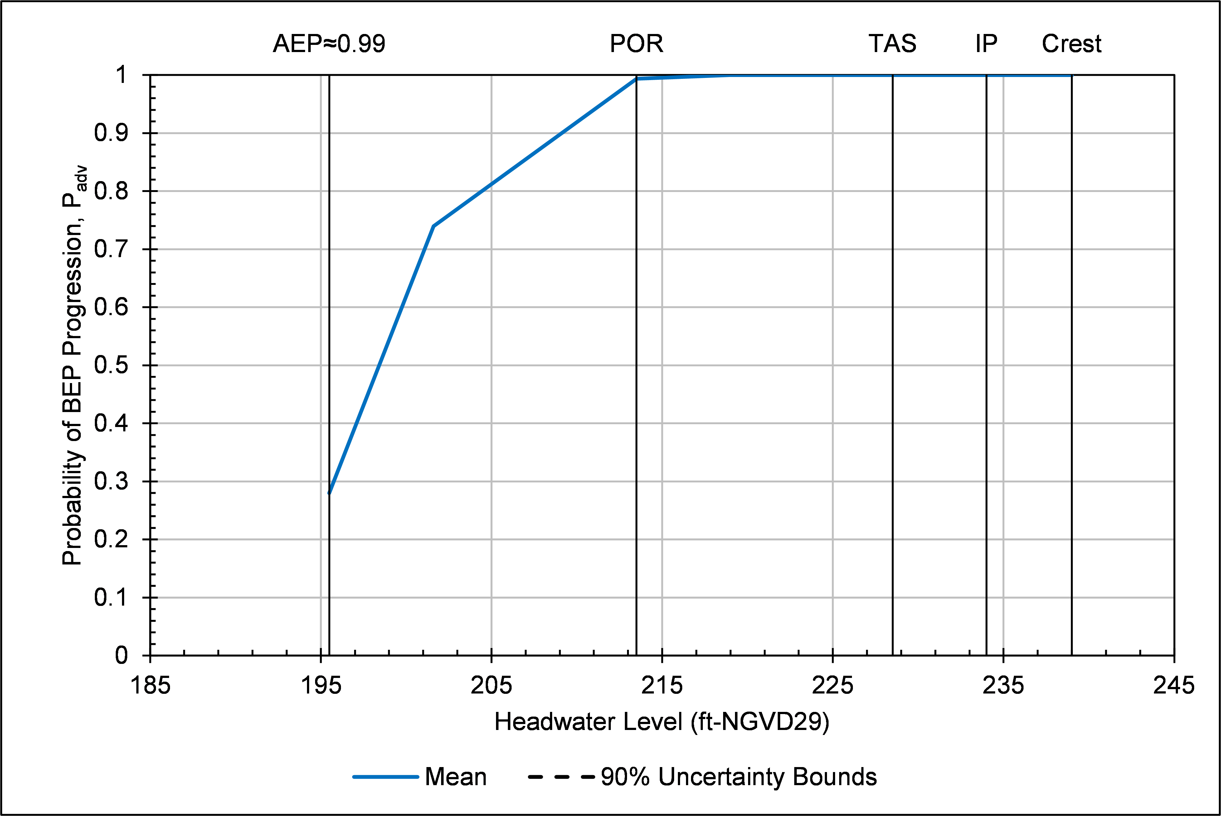
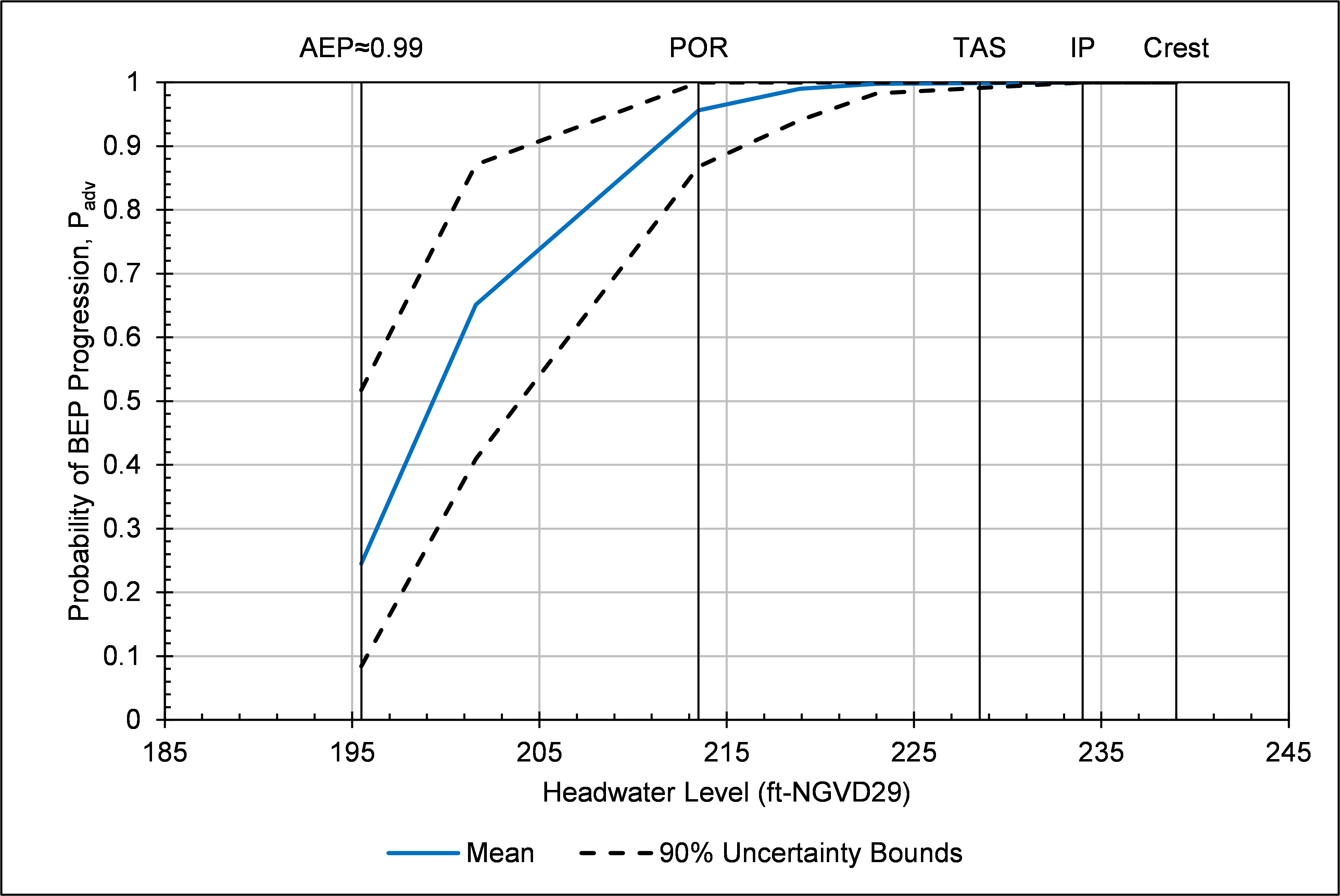
Figure illustrates the plot options for the charts in Figure and Figure. The vertical reference elevations and minimum and maximum values for the x-axis (headwater level) are the same as Figure. Only the maximum value for the y-axis (probability of BEP progression) is user-specified.

Figure: Step 7 of Schmertmann worksheet: Plot options for graphical output.