Internal Erosion Suite

Guidoux et al. Method

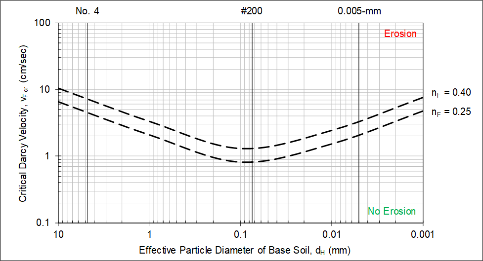
Based on experimental data, Guidoux et al. (2010) [?] proposed a relationship to estimate the critical Darcy velocity for initiation of soil contact erosion of fine soil (sand, silt, and sand/clay mixtures) below gravel as a function of effective particle diameter of the fine soil, porosity of the gravel layer, and Darcy velocity of flow through the gravel layer. In Figure, the upper relationship is for a filter (gravel layer) porosity of 0.40, and the lower relationship is for a filter (gravel layer) porosity of 0.25.

Figure: Critical Darcy velocity for Guidoux et al. (2010) method [?].

Method of Analysis

In step 1, use the drop-down list to select the method of analysis (probabilistic or deterministic). There are two options for probabilistic analysis. The first performs 1,000 iterations (judged adequate for most applications) without using Palisade’s @RISK software. This provides flexibility if an @RISK software license is not available. The second uses @RISK to customize the probabilistic analysis. Use the drop-down list to select Yes if @RISK is used and No if @RISK is not used. Figure through Figure illustrate the three possible scenarios.

Figure: Step 1 of Guidoux et al. worksheet: Deterministic analysis.

Figure: Step 1 of Guidoux et al. worksheet: Probabilistic analysis without using @RISK.

Figure: Step 1 of Guidoux et al. worksheet: Probabilistic analysis using @RISK.

Base Soil Characterization

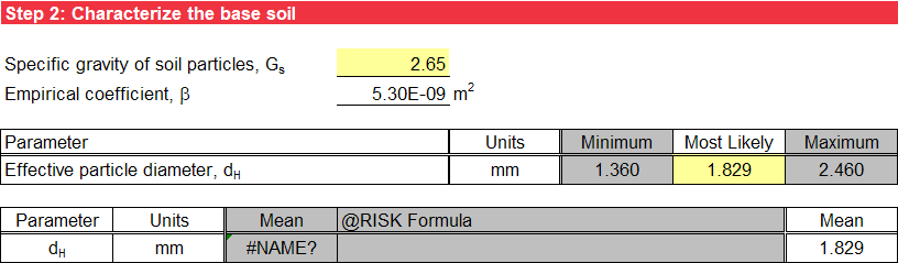
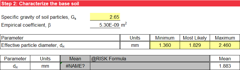
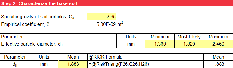
Step 2 characterizes the base soil. The input includes specific gravity of soil particles (G_s) and effective particle diameter of the base soil (d_H). The effective particle diameter of the base soil (d_H) is informed by the calculated values on the Gradation worksheet. The empirical coefficient (β) used in the equation for critical Darcy velocity is the best-fit value of 5.30E-09 m² from Guidoux et al. (2010) [?] based on experimental data.

The selections in step 1 affect the input for step 2, and cells that do not apply have a gray background. These cells are not used in subsequent calculations even if data is present.

For deterministic analysis, input only the most likely value of d_H. The mean value used for subsequent calculations is the most likely (or mode) value. Figure illustrates the deterministic input.

Figure: Step 2 of Guidoux et al. worksheet: Deterministic input.

For probabilistic analysis without using @RISK, input the minimum and maximum values in addition to the most likely value, and a triangular distribution represents d_H. The mean value used in subsequent calculations is the average of the minimum, most likely, and maximum values. Figure illustrates the probabilistic input without using @RISK.

Figure: Step 2 of Guidoux et al. worksheet: Probabilistic input without using @RISK.

For probabilistic analysis using @RISK, input the minimum, most likely, and maximum values of d_H, and use an @RISK formula for a triangular distribution in the third column as a default. Alternatively, input a valid @RISK distribution in lieu of this default formula, and the user-specified input displays in the fourth column. The mean value used in subsequent calculations is the mean for the @RISK distribution entered in the third column. Figure illustrates the probabilistic input using @RISK.

Figure: Step 2 of Guidoux et al. worksheet: Probabilistic input using @RISK.

If using @RISK to perform probabilistic analysis, delete unnecessary calculation worksheets because the simulation is performed for all worksheets in the workbook, which is time consuming. If cycling through iterations using @RISK, the displayed results are no longer mean values of the random variables; they are the selected iteration’s values.

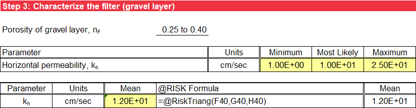
Filter (Gravel Layer) Characterization

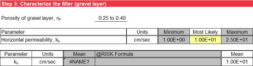
Step 3 characterizes the coarse layer. The input includes the porosity (n_F) and horizonal permeability (k_h) of the coarse layer (filter), typically gravel for this internal erosion process. A reasonable range of porosity for gravel is between 0.25 and 0.40. The coarse soils evaluated by Guidoux et al. (2010) [?] had porosity values between 0.40 and 0.43, near the upper range. However, values of porosity less than 0.40 result in lower values of critical Darcy velocity for initiation of soil contact erosion. Therefore, t critical Darcy velocity is evaluated using discrete porosity values of 0.25 and 0.40.

The selections in step 1 affect the input for step 3, and cells that do not apply have a gray background. These cells are not used in subsequent calculations even if data is present.

For deterministic analysis, input only the most likely value for k_h. The mean value used for subsequent calculations is the most likely (or mode) value. Figure illustrates the deterministic input.

Figure: Step 3 of Guidoux et al. worksheet: Deterministic input.

For probabilistic analysis without using @RISK, input the minimum and maximum values in addition to the most likely value, and a triangular distribution represents k_h. The mean value used in subsequent calculations is the average of the minimum, most likely, and maximum values. Figure illustrates the probabilistic input without using @RISK.

Figure: Step 3 of Guidoux et al. worksheet: Probabilistic input without using @RISK.

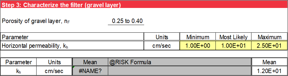
For probabilistic analysis using @RISK, input the minimum, most likely, and maximum values of k_h, and use an @RISK formula for a triangular distribution in the third column as a default. Alternatively, input a valid @RISK distribution in lieu of this default formula, and the user-specified input displays in the fourth column. The mean value used for subsequent calculations is the mean for the @RISK distribution entered in the third column. Figure illustrates the probabilistic input using @RISK.

Figure: Step 3 of Guidoux et al. worksheet: Probabilistic input using @RISK.

If using @RISK to perform probabilistic analysis, delete unnecessary calculation worksheets because the simulation is performed for all worksheets in the workbook, which is time consuming. If cycling through iterations using @RISK, the displayed results are no longer mean values of the random variables; they are the selected iteration’s values.

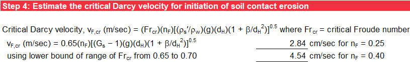
Critical Darcy Velocity for Initiation of Soil Contact Erosion

Step 4 calculates the critical Darcy velocity (v_F,_cr) for initiation of soil contact erosion for sand, silt, and sand/clay mixtures below gravel as shown in Equation.

$$v_{F,\mathrm{cr}}~(\mathrm{m/s}) = \mathrm{Fr}_{\mathrm{cr}}\, n_F\, \sqrt{ \left( \frac{\rho_s - \rho_w}{\rho_w} \right) g d_H \left( 1 + \frac{\beta}{d_H^2} \right) }$$

where:

Fr_cr = critical Froude number (0.65)
n_F = porosity of the filter (gravel layer)
ρ_s = density of the base soil particles (sand, silt, or sand/clay mixtures)
ρ_w = density of water
g = acceleration of gravity
d_H = effective particle diameter of the base soil (sand, silt, or sand/clay mixtures)
β = empirical coefficient (best fit value of 5.3E-09 m2 from experimental data)

Since it is easier to estimate the specific gravity of soil particles than the submerged density of soil particles, the following substitution in Equation is made to the equation for v_F,_cr.

$$\frac{\rho_s - \rho_w}{\rho_w} = \frac{\rho_s'}{\rho_w} = G_s - 1$$

where:

G_s = specific gravity of the base soil particles (sand, silt, or sand/clay mixtures)

Therefore, Equation shows that the equation for v_F,_cr can be simplified to:

$$v_{F,\mathrm{cr}}~(\mathrm{m/s}) = \mathrm{Fr}_{\mathrm{cr}}\, n_F\, \sqrt{ (G_s - 1)\, g\, d_H \left( 1 + \frac{\beta}{d_H^2} \right) }$$

The critical Froude number of 0.7 recommended by Guidoux et al. (2010) [?] differs from the value of 0.65 recommended by Brauns (1985) [?]. It is unclear if this is due to rounding. As previously discussed, a value of 0.65 provides a reasonable threshold for erosion and results in a lower critical Darcy velocity than Guidoux et al. (2010) [?]. Critical Darcy velocities are calculated for filter (gravel layer) porosities of 0.25 and 0.40, providing an upper and lower estimate as shown in Figure.

Based on experimental data, Guidoux et al. (2010) [?] indicated that some soils exhibited similar critical Darcy velocities for initiation of soil contact erosion despite having significantly different median particle diameters (d₅₀), while other soils exhibited similar critical Darcy velocities for initiation of soil contact erosion despite having similar d₅₀ values. Therefore, Guidoux et al. (2010) [?] concluded that d₅₀ is not a relevant soil characteristic for estimating critical Darcy velocity for fine-grained soils, and the effective particle diameter (d_H) defined by Kozeny (1953) [?] is a more representative particle-size description for a base soil.

Figure: Step 4 of Guidoux et al. worksheet: Critical Darcy velocity.

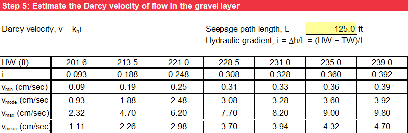
Darcy Velocity of Flow in Filter (Gravel Layer)

Step 5 calculates the average hydraulic gradient (i) of flow in the filter (gravel layer) by dividing the net hydraulic head by the user-specified seepage path length as shown in Equation.

$$i = \frac{\Delta H}{L} = \frac{\mathrm{HW} - \mathrm{TW}}{L}$$

where:

HW = headwater level
TW = tailwater level
L = seepage path length

The Darcy velocity (v) of flow in the filter (gravel layer) is calculated by multiplying the horizontal permeability of the filter (gravel layer) by the average hydraulic gradient as shown in Equation.

$$v = k_h\, i$$

where:

k_h = horizontal permeability of the filter (gravel layer)
i = hydraulic gradient in the filter (gravel layer)

The Darcy velocity for each headwater and tailwater combination is summarized in a table for the minimum, mode, maximum, and mean k_h of the filter (gravel layer), as shown in Figure. For deterministic analysis, the mean Darcy velocity is calculated using the most likely value of k_h from step 3. For probabilistic analysis without using @RISK, the mean Darcy velocity is calculated using the mean k_h obtained from a triangular distribution of the minimum, most likely, and maximum values of k_h in step 3. For probabilistic analysis using @RISK, the mean Darcy velocity is calculated using the mean k_h obtained from the user-specified distribution of the minimum, most likely, and maximum values of k_h in step 3.

Figure: Step 5 of Guidoux et al. worksheet: Darcy velocity.

Likelihood of Initiation of Soil Contact Erosion

Step 6 compares the calculated Darcy velocity of flow in the filter (gravel layer) to the critical Darcy velocity for initiation of soil contact erosion. The factor of safety (FS) against initiation of soil contact erosion is calculated as shown in Equation.

$$FS = \frac{v_{F,\mathrm{cr}}}{v}$$

where:

v_F,cr = critical Darcy velocity for initiation of soil contact erosion
v = Darcy velocity of flow in the filter (gravel layer)

For deterministic analysis, the mean Darcy velocity of flow in the filter (gravel layer) is plotted as a function of headwater level and mean effective particle diameter of the base soil (d_H). Reference lines for the critical Darcy velocity of flow through the filter (gravel layer) for porosities of 0.25 and 0.40 display as dashed lines. When a Darcy velocity at a given headwater level plots above the line of critical Darcy velocity based on the porosity of the filter (gravel layer), the FS is greater than 1, and initiation of soil contact erosion is not predicted. Figure illustrates the graphical output of Darcy velocity for deterministic analysis.

Figure: Step 6 of Guidoux et al. worksheet: Graphical output of Darcy velocity for deterministic analysis.

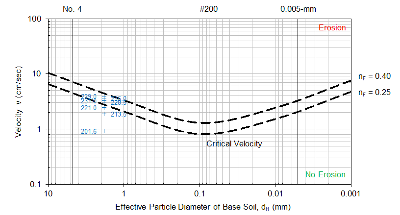
For probabilistic analysis, a black box is also plotted showing the distribution limits for effective particle diameter of the base soil and Darcy velocity of flow in the filter (gravel layer). Reference lines for the critical Darcy velocity of flow through the filter (gravel layer) for porosities of 0.25 and 0.40 display as dashed lines. Initiation of soil contact erosion is predicted for effective particle diameters and headwater combinations within the black box plotting above the line corresponding to the critical Darcy velocity being evaluated. Figure illustrates the graphical output of Darcy velocity for probabilistic analysis.

Figure: Step 6 of Guidoux et al. worksheet: Graphical output of Darcy velocity for probabilistic analysis.

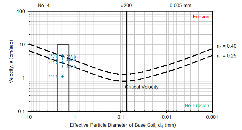
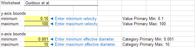
Figure illustrates the plot options for this chart. The minimum and maximum values for the y-axis (velocity) and minimum and maximum values for the x-axis (effective particle diameter of the base soil) are user-specified.

Figure: Step 6 of Guidoux et al. worksheet: Plot options of Darcy velocity for graphical output.

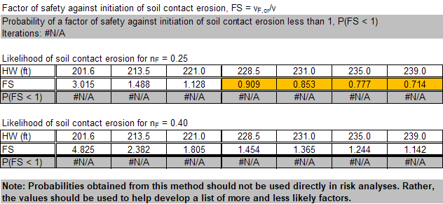
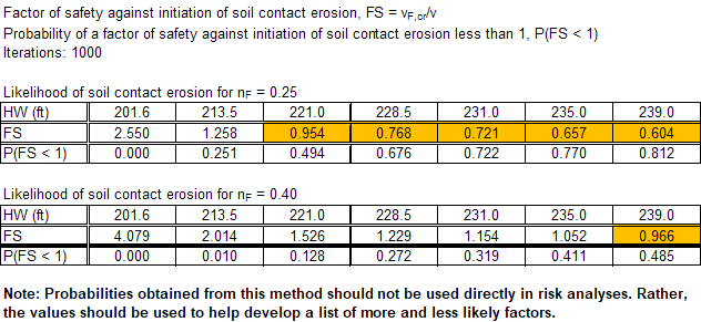
For deterministic analysis, the FS is calculated for filter (gravel layer) porosities of 0.25 and 0.40 using the most likely values of the random variables and summarized in separate tables. Cells that do not apply have a gray background. For probabilistic analysis, the FS is calculated as described for the deterministic analysis but for the mean values of the random variables, and multiple iterations are performed by sampling the distributions in step 6. The probability of initiation is equal to the percentage of iterations that resulted in a FS less than 1 [(P(FS < 1)]. For probabilistic analysis performed without using @RISK, 1,000 iterations are used. For probabilistic analysis using @RISK, the number of iterations is user-specified, and “@RISK” displays in parentheses after the number of iterations for this scenario. If cycling through iterations using @RISK, the displayed results are no longer mean values; they are the selected iteration’s values. For deterministic and probabilistic analyses, cells with FS less than 1 have an orange background. Figure illustrates the deterministic tabular output, and Figure illustrates the probabilistic tabular output without using @RISK.

Figure: Step 6 of Guidoux et al. worksheet: Tabular output for deterministic analysis.

Figure: Step 6 of Guidoux et al. worksheet: Tabular output for probabilistic analysis without using @RISK.

At the end of step 6, summary plots are generated. The first plot is the mean FS against initiation of soil contact erosion as a function of headwater level. FS is displayed for filter (gravel layer) porosities of 0.25 (blue line) and 0.40 (green line). If cycling through iterations using @RISK, the displayed results are no longer mean values; they are the selected iteration’s values. A horizontal reference line displays in black for a FS of 1.0.

Figure illustrates graphical output for deterministic analysis.

Figure: Step 6 of Guidoux et al. worksheet: Graphical output for factor of safety.

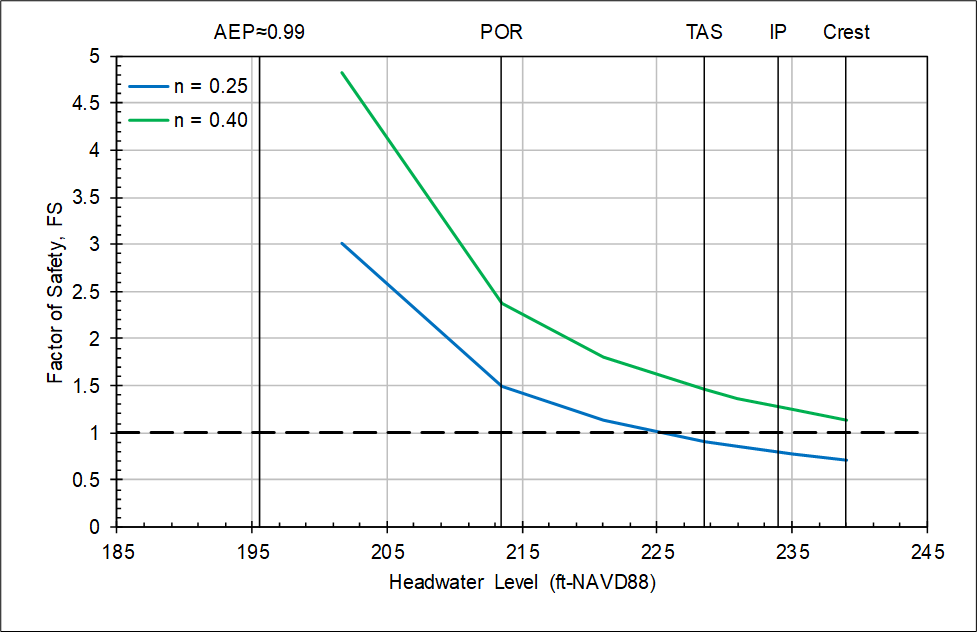
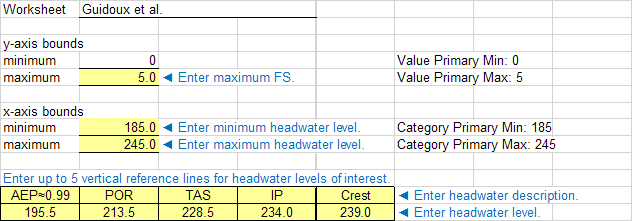
Figure illustrates the plot options for this chart. The maximum value for the y-axis (FS against initiation of soil contact erosion) and minimum and maximum values for the x-axis (headwater level) are user-specified. Users can input up to five vertical reference elevations, and user-specified labels display at the top of the chart.

Figure: Step 6 of Guidoux et al. worksheet: Plot options for factor of safety.

The second plot is the probability of initiation of soil contact erosion as a function of headwater level. For deterministic analysis, a probability of initiation of soil contact erosion is not calculated and this plot has a gray background. For probabilistic analysis, the mean probability of initiation of soil contact erosion is plotted for filter (gravel layer) porosities of 0.25 (blue line) and 0.40 (green line). If cycling through iterations using @RISK, this plot has a gray background because the probability of initiation cannot be calculated from a single iteration. Similarly, this plot has a gray background for deterministic analysis. Figure illustrates the graphical output for probabilistic analysis.

Figure: Step 6 of Guidoux et al. worksheet: Graphical output for probabilistic analysis.

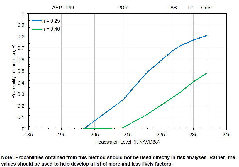
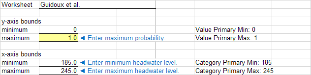
Figure illustrates the plot options for this chart. The vertical reference elevations and minimum and maximum values for the x-axis (headwater level) are the same as the previous chart. Only the maximum value for the y-axis (probability of initiation of soil contact erosion) is user-specified.

Figure: Step 6 of Guidoux et al. worksheet: Plot options for probability of initiation.

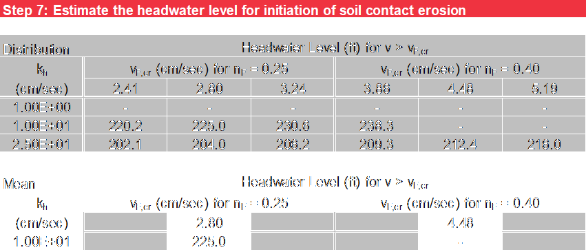
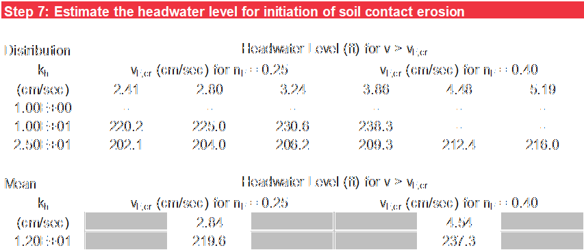
Headwater Level for Initiation of Soil Contact Erosion

Step 7 calculates the headwater level for initiation of soil contact erosion for filter (gravel layer) porosity values of 0.25 and 0.40. The results for different combinations of horizontal permeability of the filter (gravel layer) and critical Darcy velocity are linearly interpolated from the tables in step 6. The first table (Distribution) considers the combinations created by the distribution inputs in steps 2 and 3. The second table (Mean) considers the mean horizontal permeability of the filter (gravel layer) and mean critical Darcy velocity (based on effective particle diameter) and is available for both deterministic and probabilistic analyses. If the critical Darcy velocity is less than the Darcy velocity for the minimum specified headwater level, the headwater level for initiation so indicates. If the critical Darcy velocity is greater than the Darcy velocity for the maximum specified headwater level or if the Darcy velocity does not increase with an increase in headwater level (e.g., because of an increase in tailwater level), the headwater level for initiation cannot be calculated, and an error displays. For deterministic analysis, the mean value in the second table is equal to the most likely (or mode) value. Figure and Figure illustrate the critical headwater levels for deterministic and probabilistic analyses, respectively.

Figure: Step 7 of Guidoux et al. worksheet: Critical headwater level for deterministic analysis.

Figure: Step 7 of Guidoux et al. worksheet: Critical headwater level for probabilistic analysis.