Working with RMC-RFA
The following data should be gathered before creating an RMC-RFA project:
- Water control manual.
- Period of record inflow, outflow, and stage data.
- Inflow hydrograph shape, data, preferably sub-daily.
- Reservoir routing information, such as stage-storage-discharge relationships.
The following analyses should be performed external to RMC-RFA prior to creating an RMC-RFA project:
- Critical inflow duration analysis
- Volume-duration-frequency analysis
This user's manual includes limited details on the data requirements or how to perform the above analyses. For greater detail, please consult the USACE hydrologic hazard assessment methodology document An Inflow Volume-Based Approach to Estimating Stage-Frequency Curves for Dams, Bulletin 17C Guidelines for Determining Flood Flow Frequency, and Engineering Manual (EM) 1110-2-1415 Hydrologic Frequency Analysis.
- Launching RMC-RFA
- Create a New Project
- Open an Existing Project
- Input Data
- Analyses
- Reservoir Models
- Simulations
Launching RMC-RFA
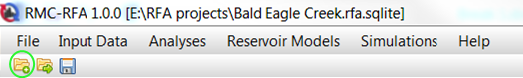
To start RMC-RFA, navigate to Documents, open the RMC-RFA folder, and select the RMC-RFA executable. If you have a shortcut created or have pinned the program to the start menu or task bar, the program can be opened by clicking on the RMC-RFA icon (Figure).
Create a New Project
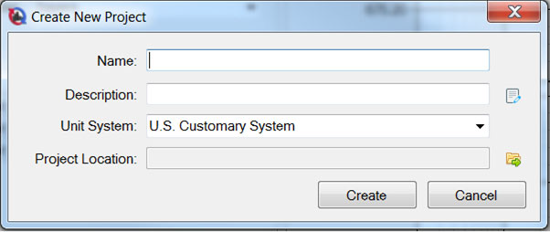
The first step in performing an analysis with RMC-RFA is to establish which directory you wish to work in and to enter a title for the new project. To start a new project, go to the File menu and select New Project. This will open the Create New Project window shown below:
A new project can also be created by clicking the New Project button in the Tool Bar.
The user is required to enter a name, select a unit system, and determine a project location. Adding a description of the study is optional, but can be beneficial. Once you have entered all the information, click Create. After clicking Create, the project name will be listed in the project explorer, and the user is ready to input data. Projects will be saved with the extension .rfa.sqlite. In a file folder they will have the project name followed by the extension.
All names must be limited to 50 characters and cannot include any special characters [!"#$%&'()*+,./:;< = >? @^`~].
Open an Existing Project
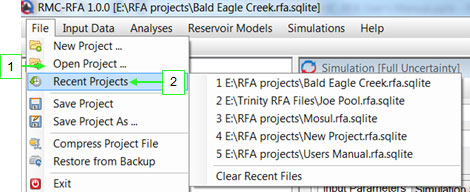
An existing project can be opened from the menu bar, by clicking File→Open Project or by selecting the project from a list of recent projects under File→Recent Projects.
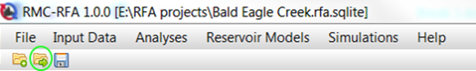
Additionally, an existing project can be opened by clicking the open project icon in the tool bar.
Managing a Project
- Rename Project
- Edit Project Description
- Change Project Unit system
Rename Project
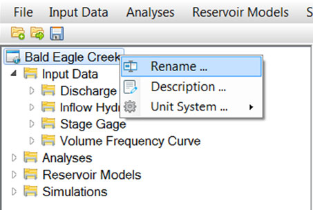
In order to rename a project, right click on the project name in the project explorer, and select Rename
The user can also rename a project from the file folder where the project is being saved. In order to do this, the project must not be opened, and the user can right click on the name and select Rename
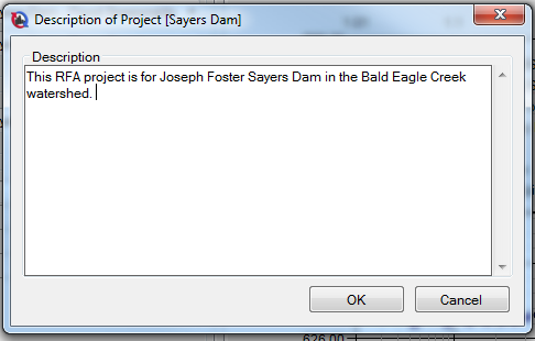
Edit Project Description
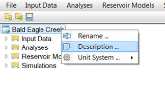
In order to edit the description on a project, right click on the project name in the project explorer and choose Description...
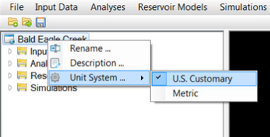
Change Project Unit System
In order to change the unit system on a project, right click on the project name in the project explorer and choose Unit System...
Managing Project Components
- Create New
- Edit
- Copy
- Rename
- Delete
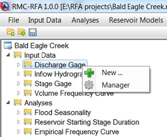
Create New
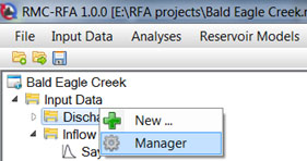
New project components can be created in two ways: For example, to enter a new discharge gage, choose Input Data -> New...-> Discharge Gage, or right click on Discharge Gage in the project explorer and select New.
- From Menu Strip
- From Project Explorer
- Choose the desired component from the menu strip.
- Select New... from the drop down menu.
- Right click on the desired project component from the project explorer.
- Select New... from the drop down menu.
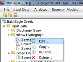
Edit
Project components can be edited in two ways:
- Right click on the item that you would like to edit from the project explorer.
- Double clicking on an item in the project explorer opens that item, or brings it to the front of the window if the item is already open.
Copy, Rename, Delete
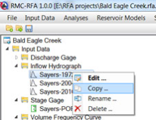
Project components can be copied in two ways:
- From Manager
- From Project Explorer
A manager is available for each category of project components. Within the manager, the user can copy a data set, rename a data set, delete a data set, or edit the description.
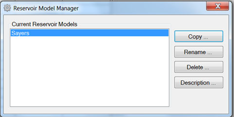
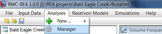
The Manager can be accessed from menu strip or the project explorer.
Right click on the item that you would like to copy, rename, or delete from the project explorer.
Input Data
There are four types of input data required for a RMC-RFA project.
- Discharge Gage
- Inflow Hydrograph
- Stage Gage
- Volume Frequency Curve
Raw data investigation is the most important step in any dam safety analysis. Many data sets have numerous occurrences of missing data, faulty data, or other issues that can impact analysis. The quality of the data that is analyzed will make the largest impact on the quality of results obtained from any computer program. In addition, know what data records are available, and how / when any operational changes have been executed. If analysis relies on a period of record, the entire dataset used needs to be homogeneous and not from mixed records or periods.
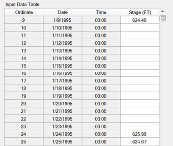
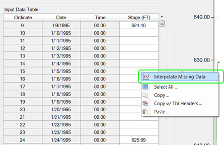
Interpolate Missing Data
Interpolate missing data is an option on the tables for discharge gage, inflow hydrograph, and stage gage. This function interpolates missing data from one defined ordinate to another along a straight line. If a second cell/ordinate is not defined, the interpolate function will fill data in to the end of the table, along a straight line interval.
Discharge Gage
The first set of data required to perform a simulation is a record of the inflows at the dam. The entire Period of Record (POR) should be used when available and appropriate. This data should be a continuous record. Note that when you create a new discharge gage, the time step option is set to 1-day and cannot be changed. This is because the discharge gage and stage gage require a mandatory 1-day time step. Daily averaged data for the POR is preferred. If the data is not in 1-day time step, it can easily be calculated from a 15-min time step or hourly time step using the math function in HEC-DSSVue. Discharge gage data is used for computing Flood Seasonality and Empirical Frequency Curves.
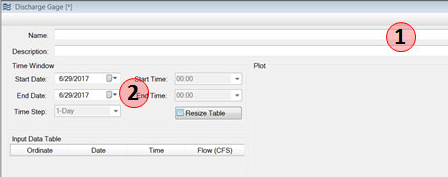
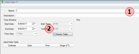
- Name and Description
- You must enter a name. All names are limited to 50 characters and cannot include the any special characters [!"#$%&'()*+,\./:;< = >? @^`{}~].
- Descriptions have no special character restrictions and allow for up to 2,000 characters, allowing a user to provide significant detail for any project component.
- Time Window
- Select a start date and an end date for the inflow data you have available.
- Hit Resize Table.
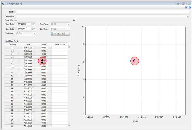
- Input Data Table
- After hitting resize table the Input Data Table will populate with ordinates, data, and time.
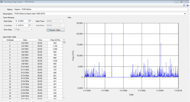
- Manually enter or copy in the flows for the entire data set.
- Plot
- When data has been entered the plot will generate. The plot has all the same features described in Chart Features.
Inflow Hydrograph
Inflow hydrographs for major historical events, large events, or synthetic events should be entered. The shape of the hydrograph is a reflection of the response of the watershed to an event. At least one inflow hydrograph shape is required to perform a simulation. Multiple inflow hydrographs can be sampled as part of the simulation. The inflow hydrograph shape is scaled up or down based on the sampled inflow volume in the stochastic simulation.
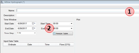
- Name and Description
- You must enter a name. All names are limited to 50 characters and cannot include the any special characters [!"#$%&'()*+,\./:;< = >? @^`{}~].
- Descriptions have no special character restrictions and allow for up to 2,000 characters, allowing a user to provide significant detail for any project component.
- Time Window
- Select a start date and an end date for the inflow hydrograph.
- Select a timestep from the drop down menu. Four time steps are available in this input data window; 15 min, 1 hour, 6 hour, and daily.
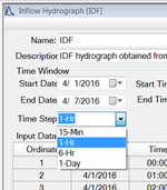
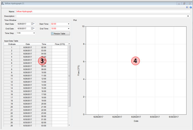
Figure: Time step options for inflow hydrographs. - Hit Resize Table.
- Input Data Table
- After hitting resize table the Input Data Table will populate with ordinates, date, and time.
- Manually enter or copy in the flows for the entire hydrograph.
- Plot
- When data has been entered the plot will generate. The plot has all the same features described in Chart Features.
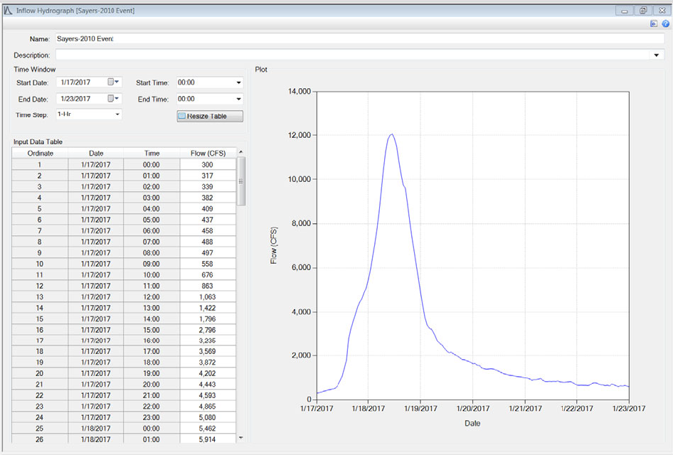
An observed inflow hydrograph from a major event should be used if at all possible. However, if no such events are available, a synthetic event, such as the Probable Maximum Flood (PMF) hydrograph may be utilized. For this type of analysis, the inflow hydrograph should be unregulated.
Verify that your inflow hydrograph shapes are inputted in one of the options for time steps. If your inflow data is in a different increment it can easily be converted to a longer duration increment using the math function "change time interval" under the tools menu in HEC-DSSVue.
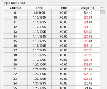
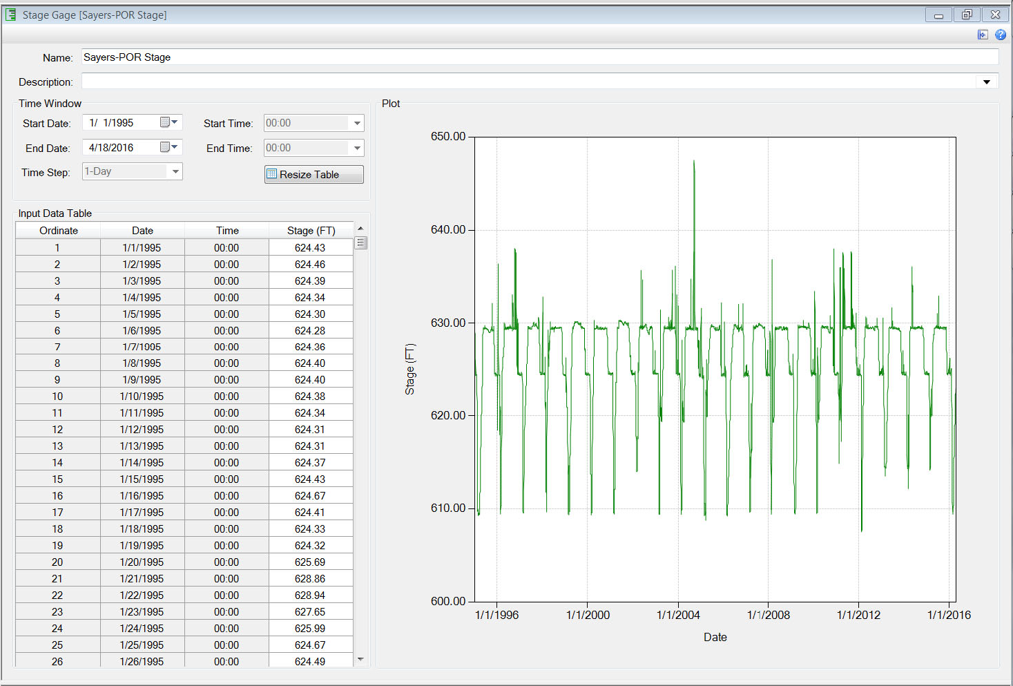
Stage Gage
For stages, the entire Period of Record (POR) for the current operation procedures should be used when available and appropriate. This data should be a continuous record. Note that when you create a new stage gage, the time step option is set to 1-day and cannot be changed. This is because the discharge gage and stage gage require a mandatory 1-day time step. Daily averaged data for the POR is preferred. If the data is not in 1-day time step, it can easily be calculated from a 15-min time step or hourly time step using the math function in HEC-DSSVue. Stage gage data is used to compute Reservoir Starting Stage Duration curves and Empirical Frequency Curves.
- Name and Description
- You must enter a name. All names are limited to 50 characters and cannot include the any special characters [!"#$%&'()*+,\./:;< = >? @^`{}~].
- Descriptions have no special character restrictions and allow for up to 2,000 characters, allowing a user to provide significant detail for any project component.
- Time Window
- Select a start date and an end date for the inflow data you have available.
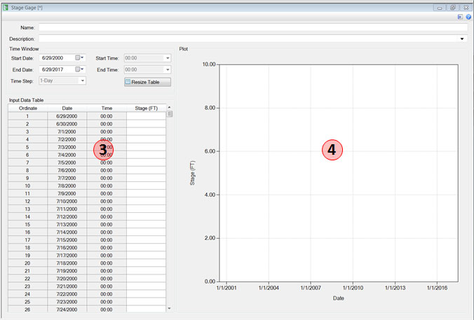
- Hit Resize Table.
- Input Data Table
- After hitting Resize Table, the Input Data Table will populate with ordinates, date, and time.
- Manually enter or copy in the stages for the entire data set.
- Plot
- When data has been entered the plot will generate. The plot has all the same features described in Chart Features.
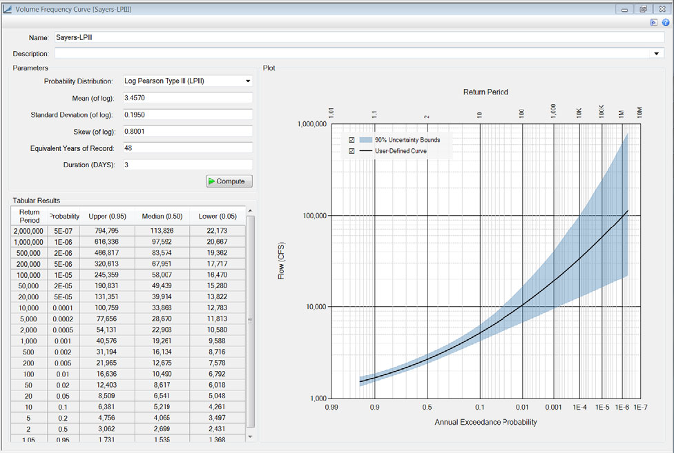
Volume Frequency Curve
Prior to creating a new volume frequency curve, the following analyses should be performed external to RMC-RFA:
- Critical inflow duration analysis
- Volume-duration-frequency analysis
For greater detail, please consult the USACE hydrologic hazard assessment methodology document An Inflow Volume-Based Approach to Estimating Stage-Frequency Curves for Dams, Bulletin 17C Guidelines for Determining Flood Flow Frequency, and Engineering Manual (EM) 1110-2-1415 Hydrologic Frequency Analysis.
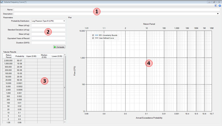
- Name & Description
- You must enter a name. All names are limited to 50 characters and cannot include the any special characters [!"#$%&'()*+,\./:;< = >? @^`{}~].
- Descriptions have no special character restrictions and allow for up to 2,000 characters, allowing a user to provide significant detail for any project component.
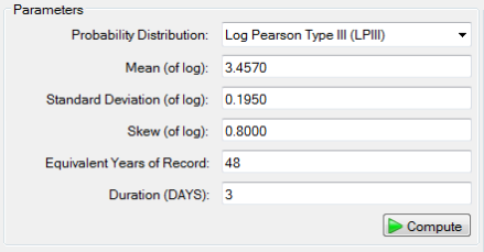
- Parameters
- Select a Probability Distribution.
- Enter distribution parameters as mean of log, standard deviation of log, and skew of log.
- Enter the equivalent years of record.
- The equivalent years of record impacts the estimated uncertainty bounds. The longer the years of record, the smaller the knowledge uncertainty in the form of sampling error. See the Basic Framework section for more detail.
- Enter the duration in days.
- The duration should correspond to the critical inflow duration, which is defined as the inflow duration that results in the highest water surface elevations for the reservoir of interest.
- After the parameters are entered, click the compute button.
- Tabular Results
- After computing the Tabular Results will be populated. RMC-RFA only provides 90% uncertainty bounds as default.
- Plot
- After computing, the Plot will be generated. RMC-RFA only provides 90% uncertainty bounds as default.
Parameters
The following parameters need to be determined before computing volume frequency curve:
- Probability Distribution
- Mean (of log)
- Standard Deviation (of log)
- Skew (of log)
- Equivalent Years of Record
- Duration
Probability Distributions
In RMC-RFA, inflow volume-frequency relationships can be defined using the Log Normal, Log Gumbel, Log Pearson Type III, or Log Generalized Extreme Value distribution, allowing the user to also assess the range of uncertainty in reservoir stage-frequency due to statistical model selection. The Log Pearson Type III distribution is the default distribution in RMC-RFA. In the current version of RMC-RFA all probability distributions require input parameters in log space.
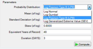
Selecting a Probability Distribution
In general, follow the guidance outlined in the USACE hydrologic hazard assessment methodology document An Inflow Volume-Based Approach to Estimating Stage-Frequency Curves for Dams, Bulletin 17C Guidelines for Determining Flood Flow Frequency, and Engineering Manual (EM) 1110-2-1415 Hydrologic Frequency Analysis. USACE recommends using the Log Pearson Type III for flow frequency. However, there are cases where a user will want to evaluate the sensitivity associated with selecting a different model. General guidance for distribution selection is provided below and summarized from Predictive Hydrology: A Frequency Analysis Approach by Meylan et al.
- Many probability distributions can be transformed by replacing the variate with its logarithmic value. The annual maximum flow series are typically not represented well by the Normal distribution. The data is skewed to right because flows are only positive in magnitude (whereas a Normal distribution will include negative flows). When the data is leftbounded (cannot be less than zero) and positively skewed, a logarithmic transformation of the data may allow the use of the Log Normal distribution. It can be argued that the occurrence of a flood results from the combination of a large number of multiplying factors (Chow, 1954) [?]. Therefore, the central limit theorem leads to the conclusion that annual maximum flows follow a Log Normal distribution because the product of n variables yields to the sum of n logarithms.
- This is a two-parameter distribution in the generalized extreme value family (EV Type 1). The Gumbel distribution is a particular case of the GEV where γ = 0 (See section on GEV below). Peak and short duration flood events It is widely used due to its ease of use.
- This distribution is also called the three-parameter Gamma distribution. Since 1967, the US water Resource Council has recommended and required the use of LPIII distributions for all US flow frequency analysis for flood insurance purposes. This distribution is flexible and usually applied to volumes corresponding to annual maximum floods. However, it should be noted that the volumes are not maximum values in the statistical sense since peak floods that are lower but of longer duration can still produce larger volumes.
- This is a flexible three-parameter distribution in the Extreme Value family that combines the Gumbel, Frechet and Weibull distribution. From the standpoint of the asymptotic theory, the GEV represents the distribution of the maximum of n random variables, and is often considered the most appropriate for modeling flow frequency.
Equivalent Years of Record
The equivalent years of record impacts the estimated uncertainty bounds. The longer the years of record, the smaller the knowledge uncertainty in the form of sampling error.
Duration
The duration should correspond to the critical inflow duration, which is defined as the inflow duration that results in the highest water surface elevations for the reservoir of interest.
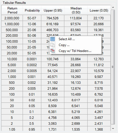
Tabular Results
Right click on the Tabular Results and a context menu will appear as shown in the figure below. The user can select all, copy, and copy with table headers. However, the user cannot paste into or edit the table data.
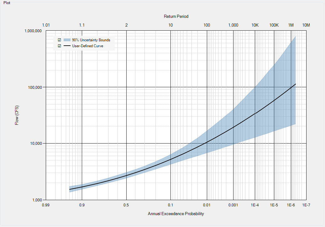
Plot
The plot displays the User-Defined Curve, and the 90% Uncertainty Bounds for the inputted volume frequency curve. This plot has all of the same features discussed in Chart Features.
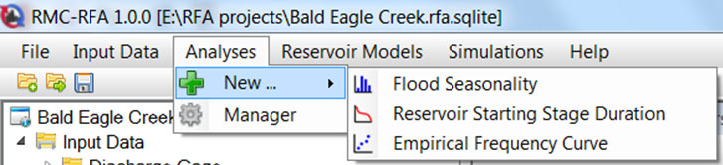
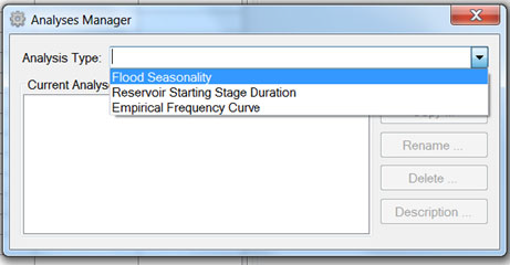
Analyses
There are three analyses that should be performed for a RMC-RFA project:
- Flood Seasonality
- Reservoir Starting Stage Duration
- Empirical Frequency Curve
Flood Seasonality
The term flood seasonality is intended to describe the frequency of occurrence of rare floods on a seasonal basis, where a rare flood is defined as any event where the flow exceeds some user specified threshold for a specified flow duration. This approach is commonly referred to as the “Peak-Over-Threshold” method.
Flood seasonality information is required in many applications in hydrology and water resources, such as seasonal streamflow forecasting, flood protection, and water resources infrastructure operations. For the purposes of the hydrologic hazard assessment of dams, flood seasonality information tells us which season an extreme flood event is most likely to occur. The information can also provide insight on mixed populations in meteorology. For example, a reservoir in the west will likely have a snowmelt season and a rainy season. Flood seasonality information can also be important if the reservoir is operated with seasonal guide curves. In many flood control reservoirs, the pool is lowered ahead of the rainy season in order to provide more storage ahead of any large flood events.
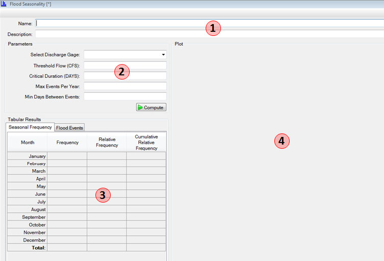
- Name & Description
- You must enter a name. All names are limited to 50 characters and cannot include the any special characters [!"#$%&'()*+,\./:;< = >? @^`{}~].
- Descriptions have no special character restrictions and allow for up to 2,000 characters, allowing a user to provide significant detail for any project component.
- Parameters
- Select a discharge gage to use in the analysis.
- Enter the threshold flow, critical duration, maximum events per year, and the minimum days between events. See the Parameters section for details.
- After the parameters are entered, click the compute button.
- Tabular Results
- After computing, the Tabular Results will be populated.
- Plot
- After computing, the Plot will be generated.
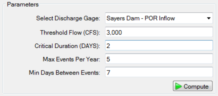
Parameters
The following parameters need to be determined before computing flood seasonality:
- Discharge Gage
- Threshold Flow
- Critical Duration
- Maximum Events Per Year
- Minimum Days Between Events
Threshold Flow
The threshold flow is usually chosen as a flow that corresponds to a specified frequency level (i.e. 2-year, 5-year or 10-year return period) for a specified critical duration to provide a common measure or rareness of the flood. There are two conflicting goals in selecting a threshold for identifying rare floods:
- The threshold needs to be high enough so that large events are considered in the analysis.
- There needs to be a dataset large enough to reduce uncertainties arising from sampling error.
Considering the two goals, the threshold needs to be set to as rare a frequency level as possible that will still provide a sufficiently large sample size. Sample sizes of 30-40 flood events are usually adequate.
Determining an appropriate threshold flow to meet this criteria is an iterative process that requires a VDF curve for the critical duration, as described in the Volume Frequency Curve section.
Critical Duration
Enter the critical duration in days. This should be the same critical duration chosen the Volume Frequency Curve. The critical duration should remain the same for the simulation.
Max Events Per Year
RMC-RFA will filter the period of record based on the threshold flow and critical duration. However, the resulting sample set may not be large enough to reduce uncertainties arising from sampling error. Therefore, in order to meet the second criterion above, a partial-duration series technique can be employed. A partial-duration series represents the occurrence of all independent events of interest, regardless of whether two or more occurred in the same year. Caution must be exercised in selecting the maximum number of events per year and the days between events to ensure the events are hydrologically independent.
Min Days Between Events
This parameter is used in conjunction with the “Maximum events per year” option. The minimum number of days between events is used to identify independent flood events. For example, if the critical inflow duration is two days, then a minimum of 7 days between events should be sufficient to ensure independence. The minimum number of days between events can also be determined by visual inspection of the flow time series to see the typical time between large flow events.
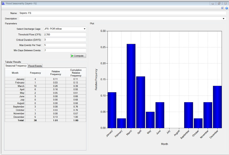
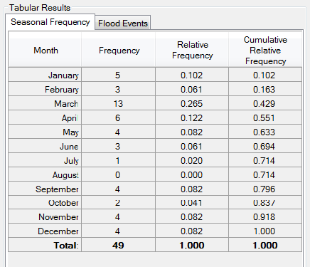
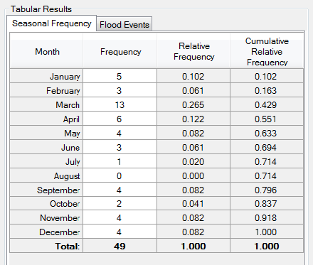
Tabular Results
The Tabular Results are presented on two tabs:
- Seasonal Frequency
- Flood Events
Seasonal Frequency
Right click on the Seasonal Frequency results and a context menu will appear as shown in the figure below.
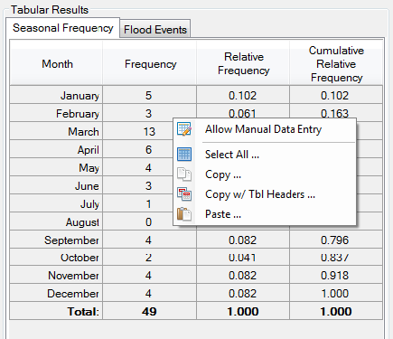
The user can choose to Allow Manual Data Entry, which will enable the user to edit the Frequency column of the Seasonal Frequency table as shown below. This option is included in RMC-RFA so that users can use flood seasonality estimates developed external of RMC-RFA.
When data has been manually entered, this will be reflected in the plot. Any manually entered storms will not appear in the Flood Events tab.
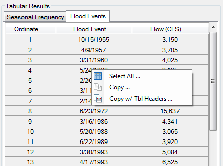
Flood Events
Right click on the Flood Events table and a context menu will appear as shown in the figure below. The user can select all, copy, and copy with table headers. However, the user cannot paste into or edit the table data.
Plot
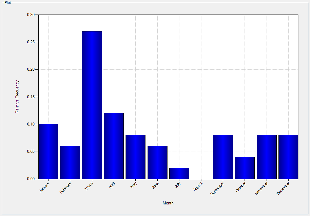
The default plot in the Flood Seasonality analysis is the relative frequency of events versus the month the event occurs. This plot has all of the same features discussed in Chart Features.
Right click on the plot and a context menu will appear as shown in the figure below.
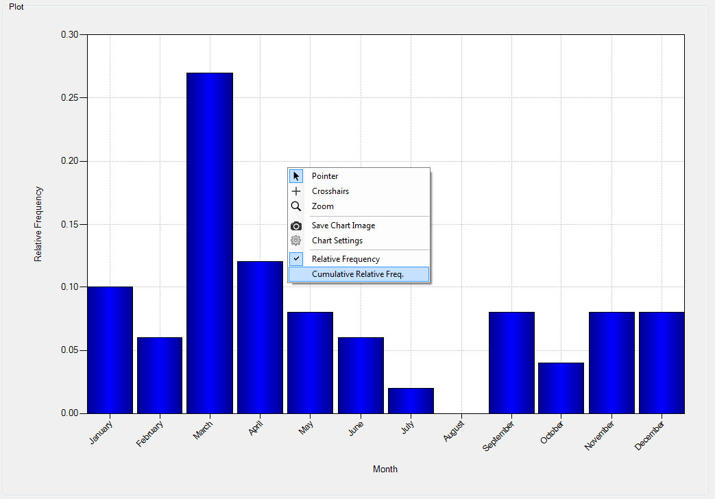
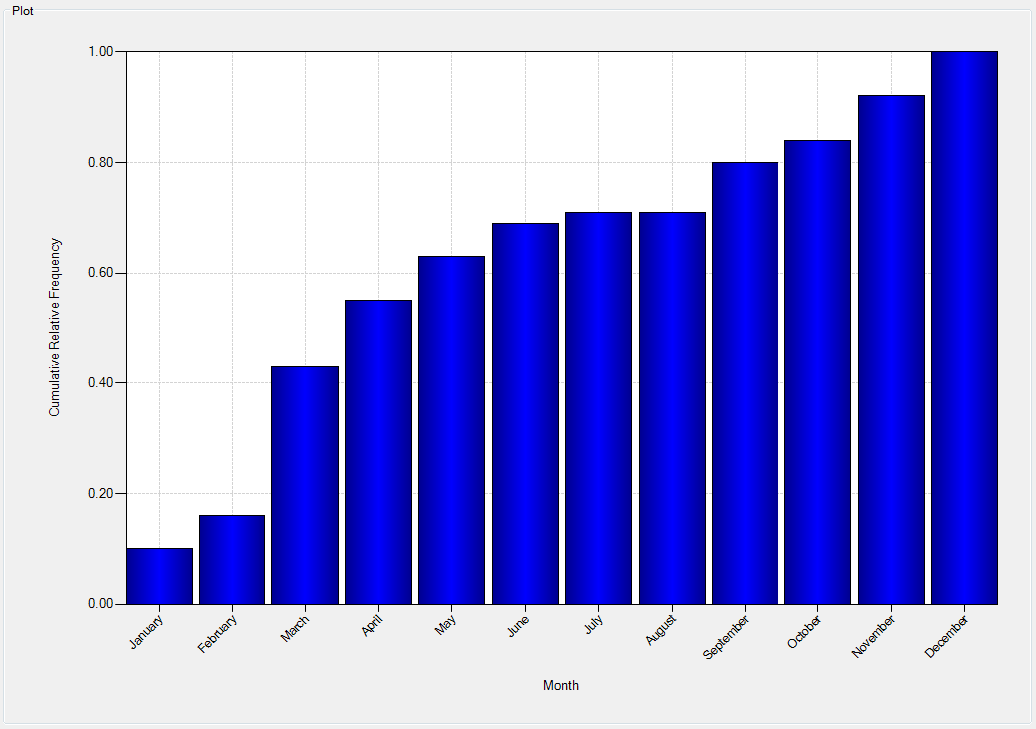
The user can choose to plot the seasonality as a cumulative relative frequency plot.
Reservoir Starting Stage Duration
Stage duration curves represent the percent of time during which specified reservoir stages are exceeded at a given location. Ordinarily, daily variations in stages are inconsequential, so duration curves are typically developed using daily average stages. Reservoir starting stage duration curves represent the percent of time during which antecedent reservoir stages are exceeded. Starting stage duration curves are developed by first filtering observed daily average stage data so that the record only contains typical starting stages based on a pool change threshold. Then, the filtered record is sorted by month or season. The filtering of the stage data is performed to avoid a certain degree of "double counting" of flood events.
In RMC-RFA, reservoir starting stage duration curves are used to derive reservoir stage-frequency curves by combining the annual exceedance probability of the inflow flood event with the probability of the stage prior to the flood event.
- Name & Description
- You must enter a name. All names are limited to 50 characters and cannot include the any special characters [!"#$%&'()*+,\./:;< = >? @^`{}~].
- Descriptions have no special character restrictions and allow for up to 2,000 characters, allowing a user to provide significant detail for any project component.
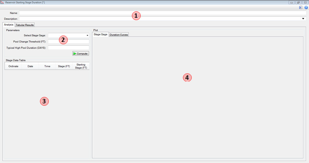
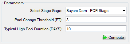
- Parameters
- Select a stage gage to use in the analysis.
- Enter the pool change threshold and the typical high pool duration. See the Parameters section for details.
- After the parameters are entered, click the compute button.
- Tabular Results
- After computing, the Tabular Results will be populated.
- Plot
- After computing, the Plot will be generated.
Parameters
The following parameters need to be determined before computing reservoir starting stage duration:
- Stage Gage
- Pool Change Threshold
- Typical High Pool Duration
Pool Change Threshold
The pool change threshold represents the maximum rate of rise of the pool per day. It will allow the starting pool elevation to be populated from daily elevations that are theorized to occur prior to any given flood event by essentially deleting all stage hydrographs that rise or fall faster than the entered threshold. If a large threshold value is chosen, you may artificially drive your starting pool too high as it takes in to account flood events where stages tend to rise quickly. An appropriate pool change threshold can by determined by visual inspection of a stage hydrograph from a normal rainfall year; i.e., a year where the reservoir was operated normally because there was no significant flood events.
First, inspect the period of record. Choose a year without a significant event and inspect the stage hydrograph from that year. You can then estimate the rate of pool change per day from the hydrograph. It may be beneficial to review several normal years and take an average daily rate of rise. The normal rate of rise can be compared to a hydrograph from an event year where the stage should be rising much faster.
For example, the Joseph Foster Sayers Dam stage hydrograph below is taken from the spring of 1999, a normal precipitation year. The rate of rise per day is shown in below. The maximum rate of rise is about 2 feet. After repeating this process for the years 2000 and 2001, also years with normal rainfall, it is determined that approximately 2 feet is indeed a good estimation for maximum normal rate of rise for this project.
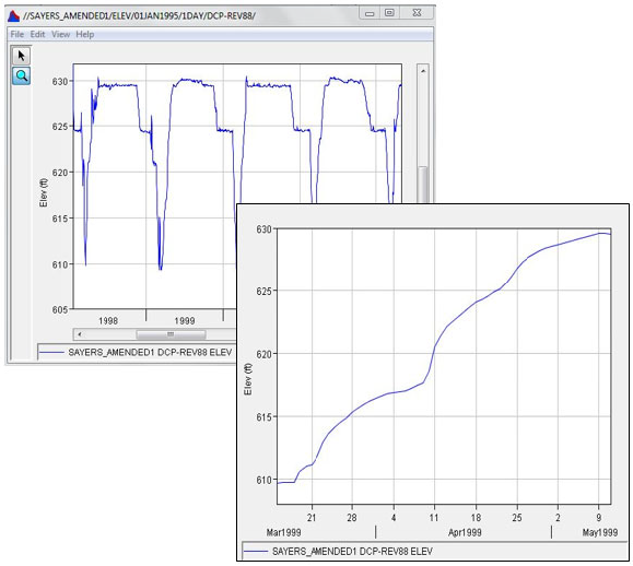
| Ordinate | Date | Stage (ft) | Rate of Change |
|---|---|---|---|
| 17 | 30Mar1999 | 616.25 | 0.172 |
| 18 | 31Mar1999 | 616.42 | 0.210 |
| 19 | 01Apr1999 | 616.63 | 0.180 |
| 20 | 02Apr1999 | 616.81 | 0.086 |
| 21 | 03Apr1999 | 616.90 | 0.074 |
| 22 | 04Apr1999 | 616.97 | 0.076 |
| 23 | 05Apr1999 | 617.05 | 0.162 |
| 24 | 06Apr1999 | 617.21 | 0.240 |
| 25 | 07Apr1999 | 617.45 | 0.240 |
| 26 | 08Apr1999 | 617.69 | 0.876 |
| 27 | 09Apr1999 | 618.56 | 1.938 |
| 28 | 10Apr1999 | 620.50 | 0.892 |
| 29 | 11Apr1999 | 621.39 | 0.720 |
As you can see in the figure below, the hydrograph taken from the September 2004 shows a much faster rate of rise, consistent with a flood event. Sensitivity runs should be made to determine the appropriate threshold that meets the above criteria.
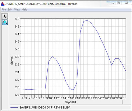
| Ordinate | Date | Stage (ft) | Rate of Change |
|---|---|---|---|
| 17 | 16Sep2004 | 629.14 | 1.830 |
| 18 | 17Sep2004 | 630.97 | 13.535 |
| 19 | 18Sep2004 | 644.51 | 2.755 |
| 20 | 19Sep2004 | 647.26 | 0.270 |
Setting the pool change threshold to zero will result in no filtered stage gage date: i.e., stage duration curves will be constructed from the full period of record.
Typical High Pool Duration
Similar to the Pool Change Threshold, the high pool duration is another parameter used to filter out large events for the purpose of distilling the record to only the typical starting pool elevations. It too can be determined by visual inspection. In this case, chose an event stage hydrograph and visually inspect how many days the high pool typically lasts. Again, it may be beneficial to analyze several event hydrographs, if they are available, and take an average of the high pool durations.
Tabular Results
The Tabular Results are provided in two sections:
- Stage Data Table
- Tabular Results
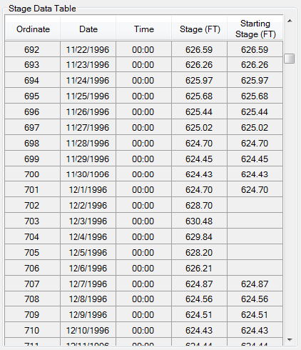
Stage Data Table
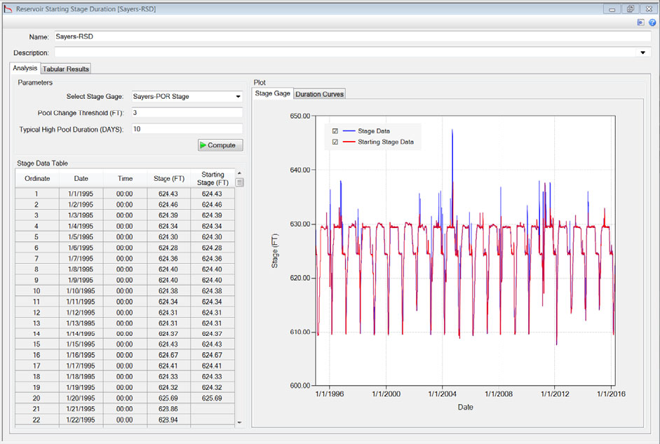
The raw stage gage data along with the filtered starting stage data are reported in the Stage Data Table as shown below.
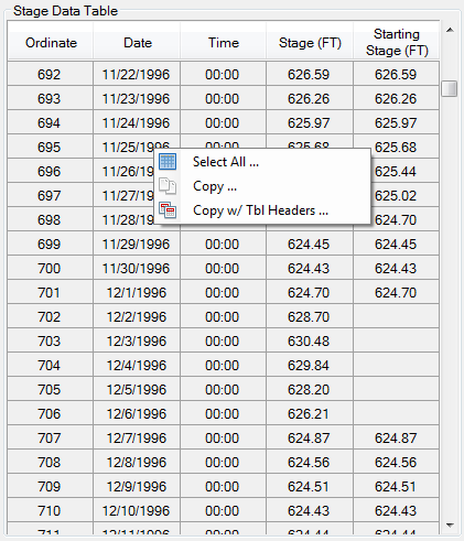
Right click on the Stage Data Table and a context menu will appear as shown in the figure below.
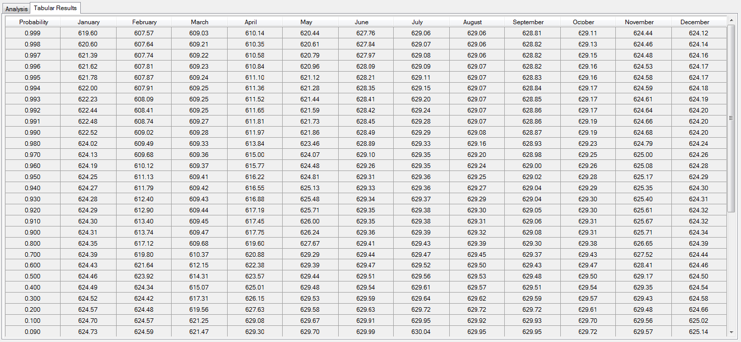
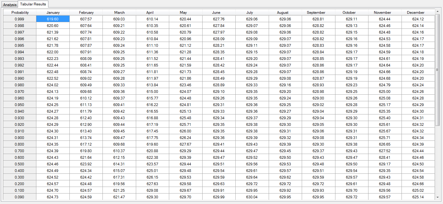
Tabular Results
Reservoir starting stage duration curves are provided in the Tabular Results tab as shown below.
Right click on the Tabular Results and a context menu will appear as shown in the figure below.
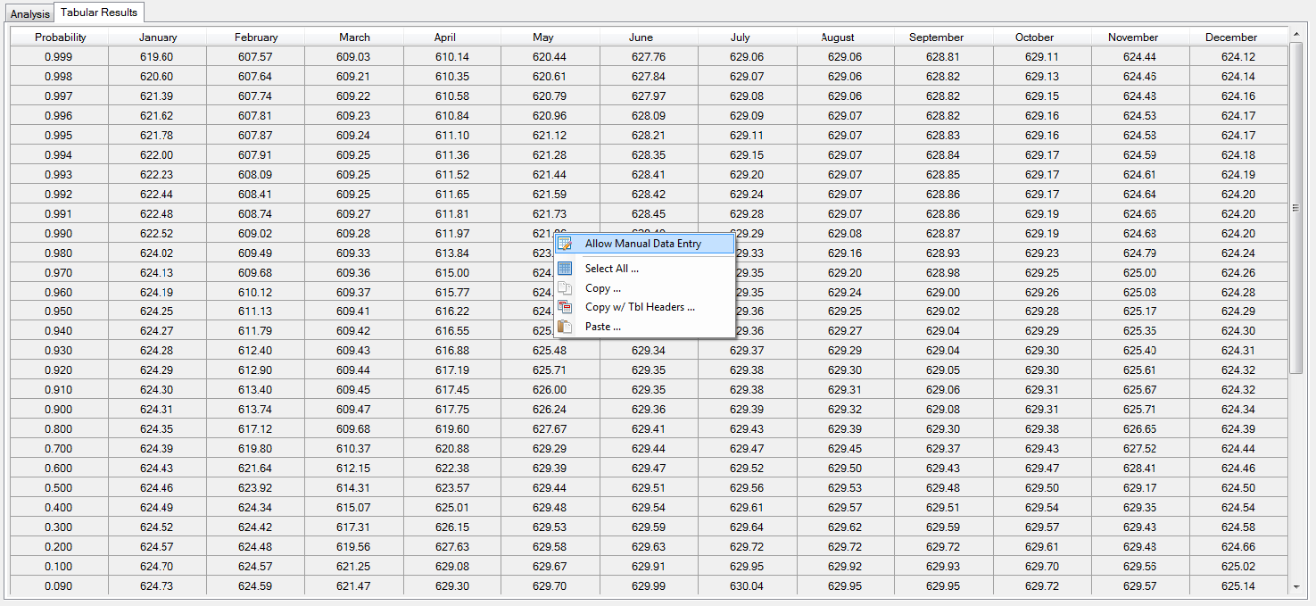
The user can choose to Allow Manual Data Entry, which will enable the user to edit the duration curves as shown below. This option is included in RMC-RFA so that users can use starting duration estimates developed external of RMC-RFA.
Plot
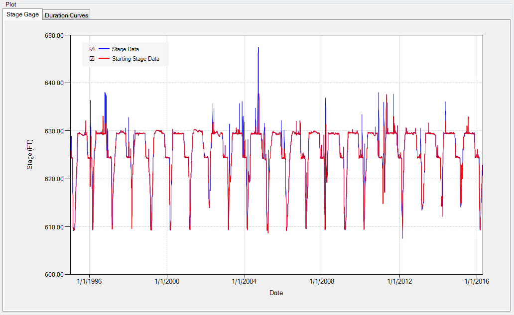
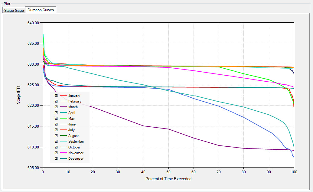
There are two plots provided in a reservoir stage duration analysis (both plots have all of the same features discussed in Chart Features):
- Stage Gage
- Duration Curves
The Stage Gage plot illustrates the effect of the selected filtering Parameters as shown below.
The Duration Curves plot illustrates the resulting starting stage duration curves as shown below.
Empirical Frequency Curve
For the evaluation of hydrologic hazards, an extreme-value series of annual maximum discharges or stages can be generated from the observed period of record. An empirical frequency is constructed by the ranking annual maximum data in descending order, assigning the data a plotting position, and then plotting the data on a probability plot.
- Name & Description
- You must enter a name. All names are limited to 50 characters and cannot include any special characters [!"#$%&'()*+,\./:;< = >? @^`{}~].
- Descriptions have no special character restrictions and allow for up to 2,000 characters, allowing a user to provide significant detail for any project component.
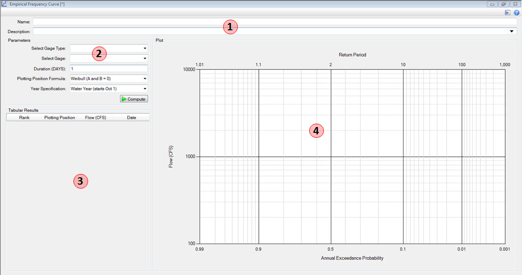
- Parameters
- Select a stage gage to use in the analysis.
- Enter the duration, and select a plotting position and year specification. See the Parameters section for details.
- After the parameters are entered, click the compute button.
- Tabular Results
- After computing, the Tabular Results will be populated.
- Plot
- After computing, the Plot will be generated.
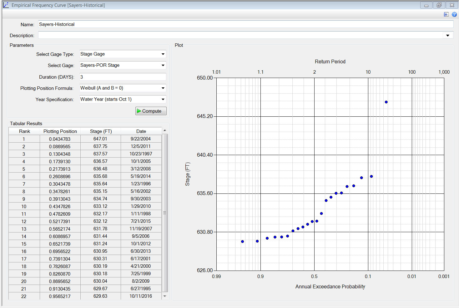
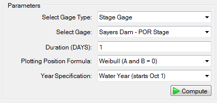
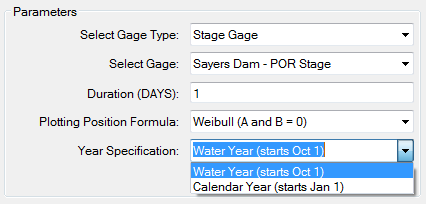
Parameters
The following parameters need to be determined before computing empirical frequency curve:
- Gage Type (either Discharge or Stage)
- Gage
- Duration
- Plotting Position formula
- Year Specification
Duration
Annual maximum values will extracted for the specified duration. If a discharge gage representing inflow to the reservoir is selected, then the duration could be the critical inflow duration, which is defined as the inflow duration that results in the highest water surface elevations for the reservoir of interest. Whereas, if the discharge gage represents outflow, the specified duration could be the duration likely to cause spillway erosion. If a stage gage is selected, the duration should be set to 1 in order to capture peak stages for comparison in a Simulation.
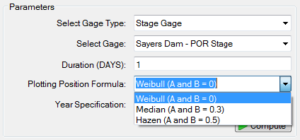
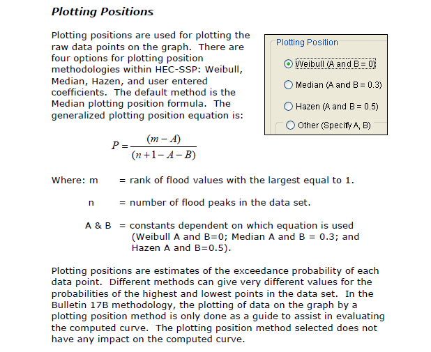
Plotting Position Formulas
There are a number of plotting position formulas for the estimation of empirical frequency. The formulas compute the exceedance probability of a data point based on the rank of the data point in a sample of a given size. Among different formulas, the differences in estimated exceedance frequency for each data point is minor for ranks of 3 and lower (the third largest value and all smaller values.) For the largest observation in the set (rank 1) the difference can be quite large.
In RMC-RFA, there are three plotting positions available for selection in the empirical frequency curve analysis:
- Weibull (A and B = 0), which is the default
- Median (A and N = 0.3)
- Hazen (A and B = 0.5)
The HEC-SSP user's manual provides a great summary of plotting positions as shown below:
Year Specification
This option allows the user to define the beginning and ending date for the analysis year for ranking data. These dates are used for extracting annual maximum discharges or stages. It is important to choose a year specification that captures all flood events from a specific hydrologic regime. For example, if the flood season typically occurs in the spring and summer, then a calendar year (starts Jan 1) specification would sufficiently capture those events. However, if the flood season occurs in the fall and winter, then a water year (starts Oct 1) specification would better capture those events.
In RMC-RFA, there are two year specifications available for selection in the empirical frequency curve analysis:
- Water Year (starts Oct 1), which is the default
- Calendar Year (starts Jan 1)
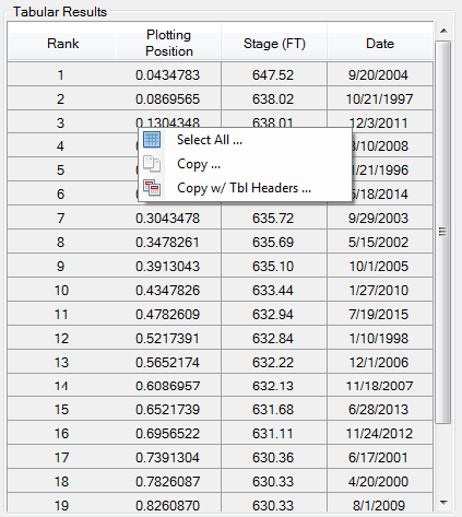
Tabular Results
Right click on the Tabular Results and a context menu will appear as shown in the figure below. The user can select all, copy, and copy with table headers. However, the user cannot paste into or edit the table data.
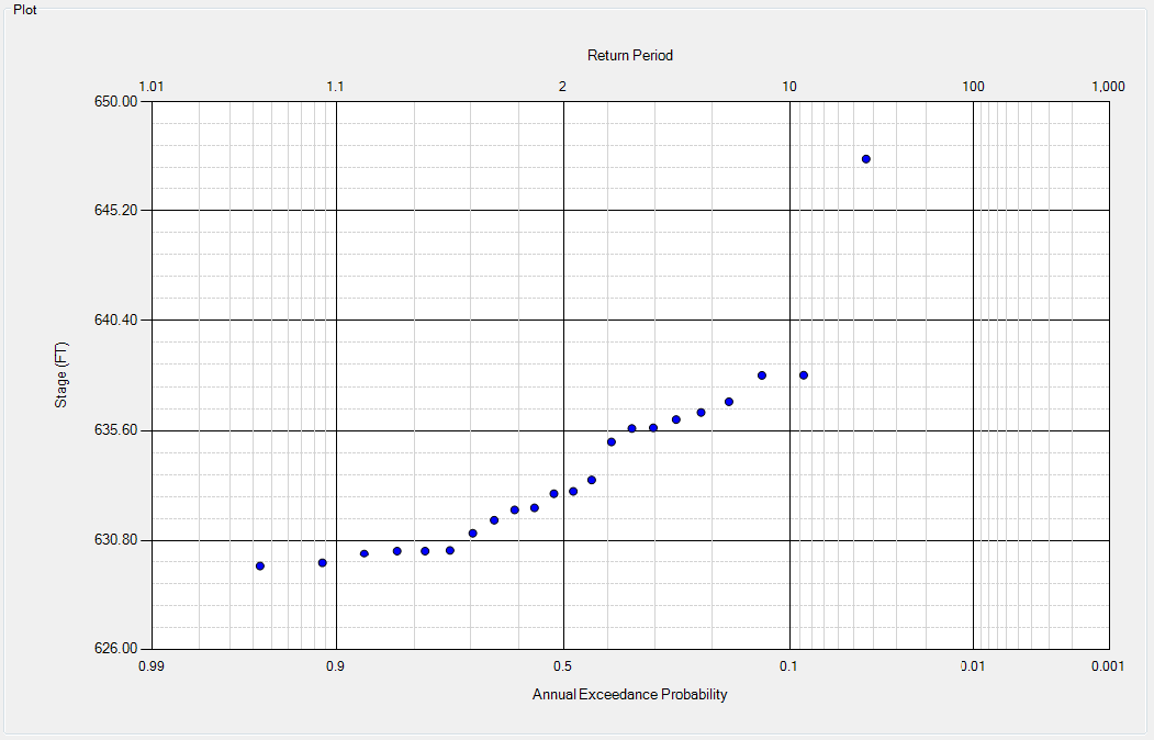
Plot
The plot in the Flood Seasonality analysis is the relative frequency of events versus the month the event occurs. This plot has all of the same features discussed in Chart Features.
Reservoir Models
A reservoir routing model is used to determine pool stages and discharges by routing a flood hydrograph through the reservoir pool and outlets. The reservoir routing model includes characteristics of the reservoir, such as the stage-storage relationship, and information about physical structures, like spillways and other outlets. These regulating outlets are commonly simplified within a stage-storage-discharge relationship.
RMC-RFA allows a user to create more than one reservoir model, if desired, allowing the user to look at routing results using different operational scenarios. For example, the user could create one stage-storage-discharge function associated with spillway operations only, and a second corresponding to spillway operations and gate operations. This would allow comparison of simulation with and without gates operable.
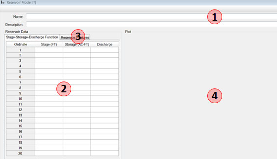
- Name & Description
- You must enter a name. All names are limited to 50 characters and cannot include the any special characters [!"#$%&'()*+,\./:;< = >? @^`{}~].
- Descriptions have no special character restrictions and allow for up to 2,000 characters, allowing a user to provide significant detail for any project component.
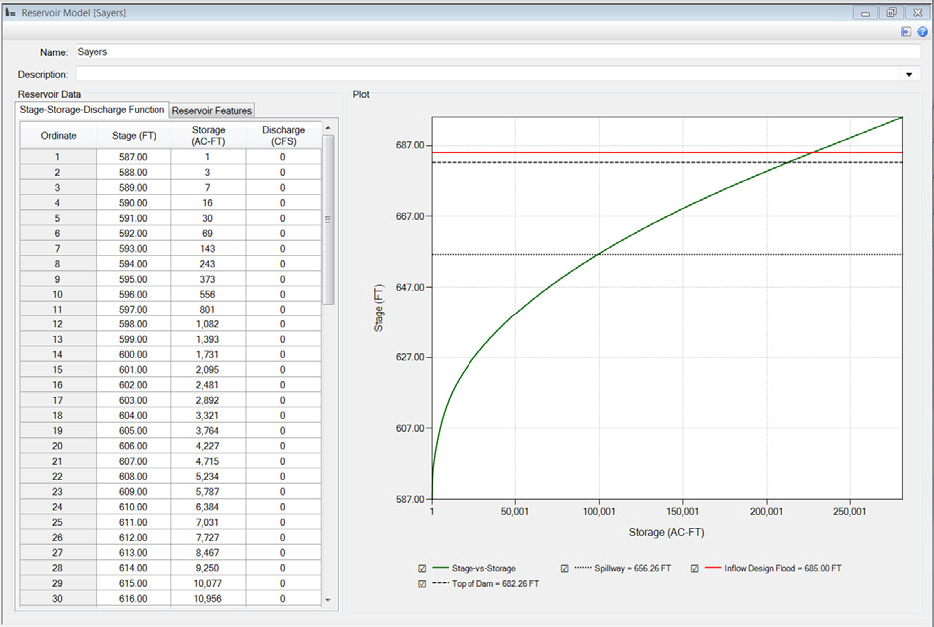
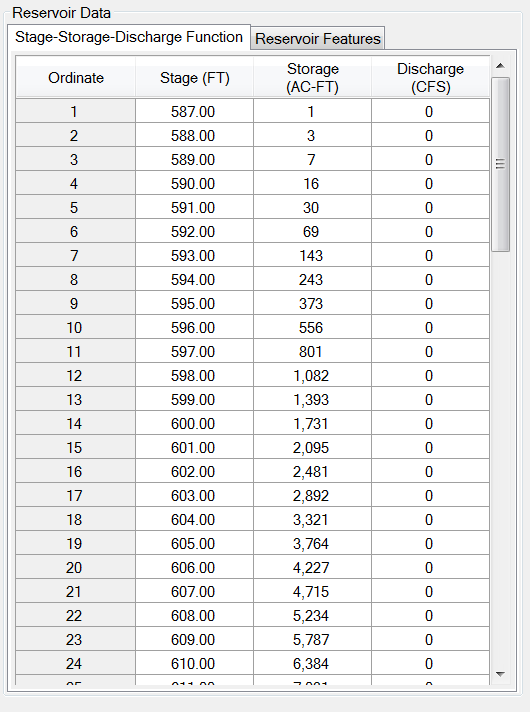
- Reservoir Data: Stage-Storage-Discharge Function
- Enter the stage, storage, and associated discharge into the table. See Stage-Storage-Discharge Function.
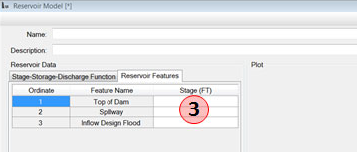
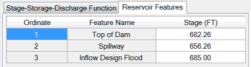
- Reservoir Data: Reservoir Features
- Click on the next tab in reservoir data.
- Enter the top of dam, spillway, and inflow design flood stage.
- Plot
- After entering the reservoir data, the Plot will be generated.
Stage-Storage-Discharge Function
Modified Puls Routing
Reservoir routing in RMC-RFA is based on a "hydrologic method", which is concentrated on the concept of storage for the flood water and does not directly include effects of resistance to the flow. The routing of a flood by using a hydrologic method in a given reservoir is based on the continuity equation which equates the rate of change of the storage, in the reservoir to the difference between the inflow, I, and outflow, O:
Specifically, RMC-RFA uses a finite difference approximation of the continuity equation called the Modified Puls routing method, also known as storage routing or level-pool routing. Using a simple backward differencing scheme and rearranging the continuity equation to isolate the unknown values gives:
where:
and = inflow hydrograph ordinates at times and , respectively
and = outflow hydrograph ordinates at times and , respectively
and = storage in the reservoir at times and , respectively
The Modified Puls method has some limitations, which includes among others rivers with significant backwater effects, tributary inflows, and flat to mild channel slopes. If the dam being assessed has a long and narrow reservoir or has a potential for significant backwater effects, the Modified Puls routing method included in RMC-RFA may not provide accurate results for peak stage.
Stage versus Storage Volume
A stage versus storage relationship (also referred to as a stage-storage function) relates water surface elevation to the volume of water stored. It provides a geometric description of the reservoir that is used during routing to determine the rise or fall of the water surface elevation given a change in the volume of stored water. In most cases, a stage-storage curve will be provided in the project water control manual or can be attained from the dam owner, such as the Corps District. In some cases, the water control manual will only provide a stage-area relationship, which can also be used to develop a stage-storage relationship.
Stage versus Discharge
A stage versus discharge relationship (also referred to as a stage-discharge function) relates water surface elevation to the required discharge associated with the outlet works, spillway or overtopping. Stage-discharge information will be provided in the project water control manual. The stage-discharge relationship should encompass any releases from the dam, including outlet works, spillways, and overtopping if necessary. Overtopping discharges should be included in the stage-discharge relationship in order to properly capture extreme flood events that result in overtopping. For additional details on stage versus storage and stage versus discharge, refer to "An Inflow Volume-Based Approach to Estimating Stage-Frequency Curves for Dams"
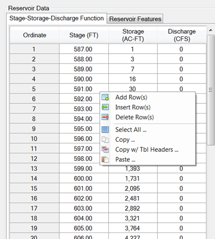
In the stage-storage-discharge table, the user can add rows, insert rows, delete rows, select all, copy, copy with table headers and paste by right clicking within the table.
Reservoir Features
Enter the stage for the top of dam, spillway, and inflow design flood. These reservoir features are used as reference points to aid with interpretation of simulation results.
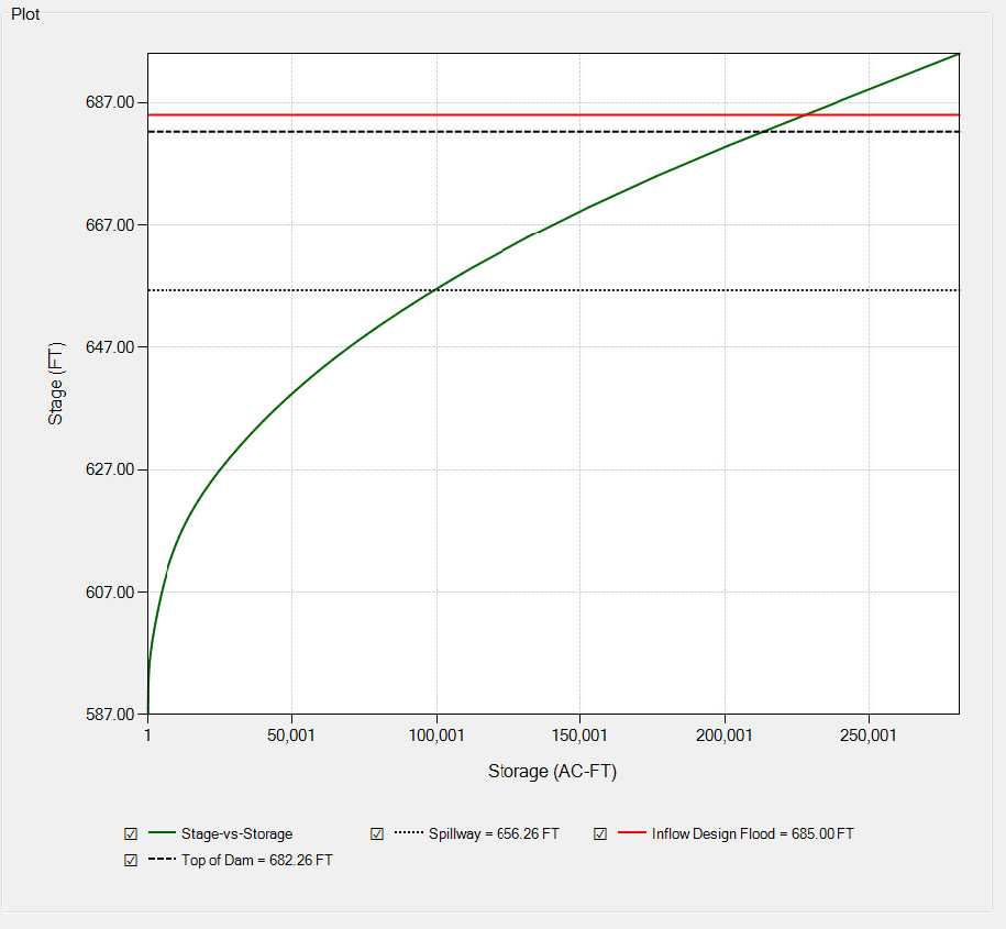
Plot
The default plot in the Reservoir Model is the stage-storage-discharge curve. It also displays the Reservoir Features. This plot has all of the same features discussed in Chart Features.
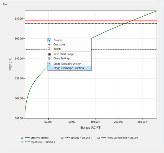
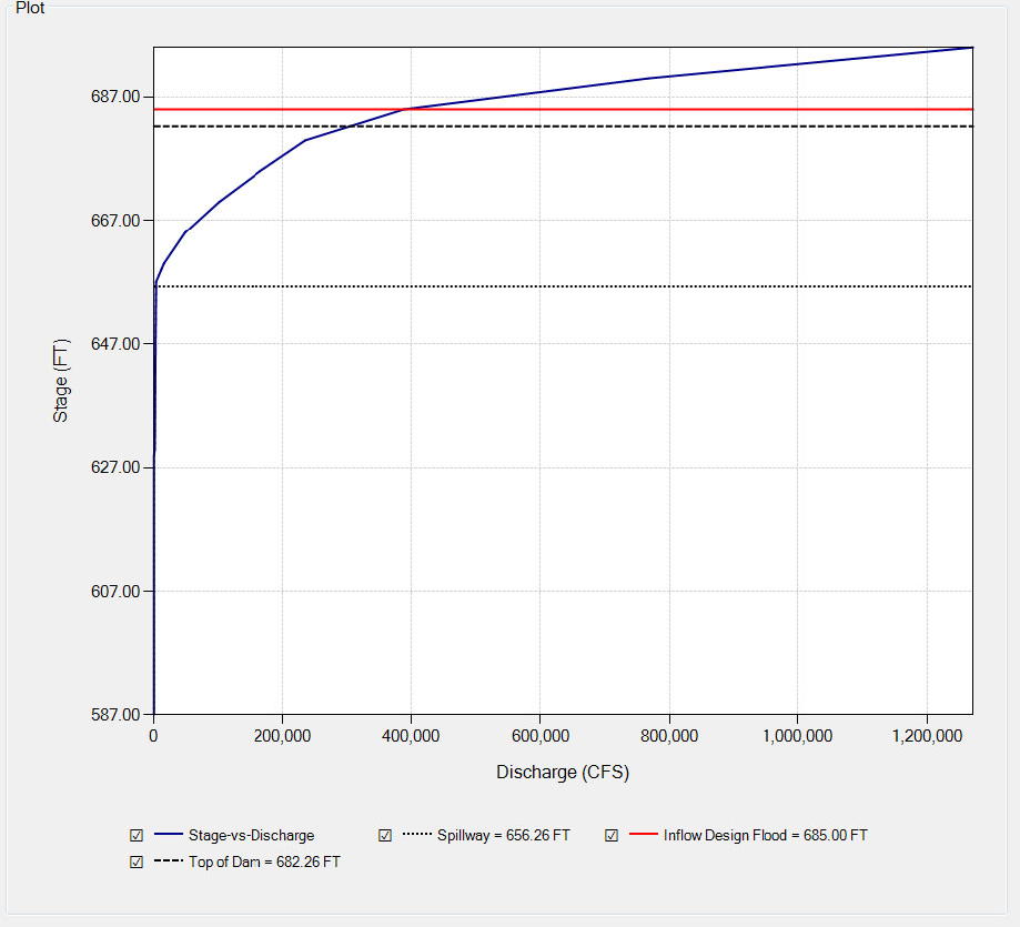
Right clicking within the plot allows the user to select the stage-discharge function plot.
Simulations
Simulations incorporate the input data, analyses, and reservoir models in order to perform the stochastic simulation.
- Name & Description
- You must enter a name. All names are limited to 50 characters and cannot include the any special characters [!"#$%&'()*+,\./:;< = >? @^`{}~].
- Descriptions have no special character restrictions and allow for up to 2,000 characters, allowing a user to provide significant detail for any project component.
- Simulation Parameters
- Enter all required Simulation Parameters.
- After entering all required information hit Simulate button.
- The project will automatically save any changes and begin the simulation. If the simulation does not begin, check the message window for any warnings indicating why the simulation was not successful.
- While a simulation is being performed, the user can cancel the simulation at any time using the Cancel button.
- While the simulation is being performed, a progress bar appears to the left of the simulate button showing the progress of the simulation.
- When simulation is complete the following image will appear:
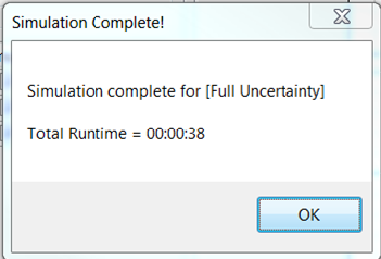
Figure: Simulation complete window. - Tabular Results
- Tabular Results are generated after a simulation. Click on the Tabular Results tab to display these results.
- Plots
- Plots are generated after a simulation. There are four main categories of plots: Frequency Curve Plots, Simulated Input Plots, Sensitivity Plots, and Routed Hydrograph Plots.
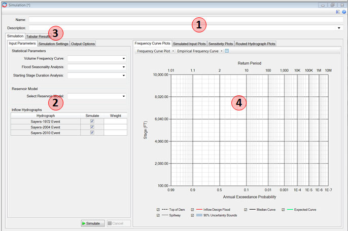
Simulation Parameters
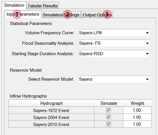
- Input Parameters
- Select a volume frequency curve, a flood seasonality analysis, a starting stage duration analysis, and a reservoir model analysis. For details see Input Parameters.
- Select which inflow hydrographs to include in the simulation and assign them a weight.
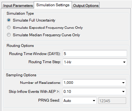
- Simulation Settings
- Select the Simulations Settings tab.
- Select a Simulation type.
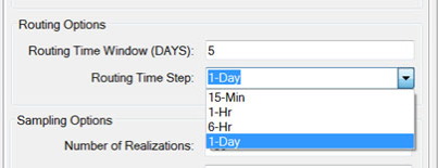
- Enter the Routing Options: the routing time window in days and the routing time step.
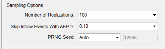
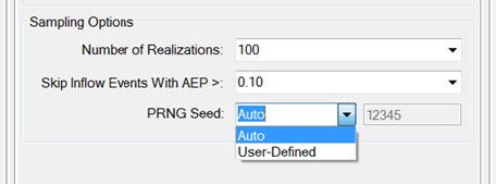
- Select Sampling Options: the Number of Realizations, Skip Inflow Events With AEP, and PRNG Seed.
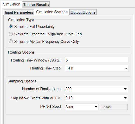
Figure: Simulation settings tab. - Output Options
- Select the Output Options tab.
- Determine which Frequency Curves you would like the simulation to create.
- Set an Uncertainty Bound.
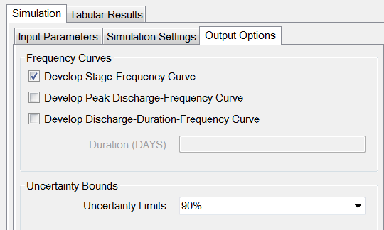
Figure: Output options tab.
Input Parameters
Input Parameters is where the user selects the parameters to be used in a simulation.
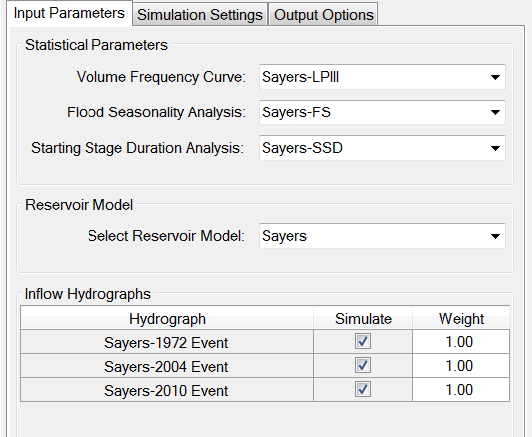
The Statistical Parameters are the Volume Frequency Curve, Flood Seasonality Analysis, and the Starting Stage Duration Analysis. The drop down menu associated with each of these items will show the names of the analyses performed under the analyses tab. Reservoir Model allows the user to select one of the reservoir models they have created. Selecting a reservoir model will populate the plot with the dam features. Finally the user choses which Inflow Hydrograph to use for the simulation, and assigns the inflow hydrograph a weight to influence how often it is used in the simulation. You can perform a simulation with as little as one inflow hydrograph.
The weight assigned to each inflow hydrograph determines how often that particular hydrograph will be sampled in the simulation. The weighting needs to be numeric. The weights do not need to sum to 1. Instead, the weights are normalized at the start of the simulation. For example if you have two hydrographs, and assign one a weight of 1 and the second a weight of 2, then the first hydrograph will be sampled 1/3 of the time, and the second hydrograph will be sampled 2/3 of the time.
RMC-RFA will scale the input hydrograph shape to match the sampled inflow volume based on the selected critical duration defined in the Volume Frequency Curve input.
Simulation Settings
Simulation settings determine the simulation type, routing options, and sampling options and has a large influence on how long the simulation will take to perform.
- Simulation Type
- Routing Options
- Sampling Options
Simulation Type
Three options are available for simulation type:
- Simulate Full Uncertainty
- Simulate Expected Frequency Curve Only
- Simulate Median Frequency Curve Only
For rapid sensitivity analysis, the user should select either Simulate Expected Frequency Curve Only or Simulate Median Frequency Curve Only as run times are much shorter. Simulate Full Uncertainty will have the longest run time, as it calculates the Median Curve, Expected Curve, and Uncertainty Bounds.
Routing Options
Routing Time Window (DAYS): This indicates the number of days to route the simulation. This value should be at least as long as the critical inflow duration defined by the Volume Frequency Curve input. The routing time window needs to be long enough to ensure the reservoir stage has had enough time to crest.
Routing Time Step: A drop down menu, allowing the user to choose from the following simulation time steps: 15-min, 1-Hr, 6-Hr, and 1-Day. The routing time step chosen will affect the simulation run time (e.g., a simulation with a 15-Min time step will take about four times longer than a simulation with a 1-Hr time step).
Sampling Options
- Number of Realizations
- Skip Inflow Events
- PRNG Seed
Number of Realizations
This is a drop down menu, allowing the user to choose the number of realizations to perform in the simulation. The number of realization options can be seen in the figure below.
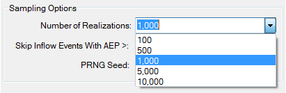
The number of realizations should be chosen with consideration of run time, accuracy, and project needs. Often, a user will run the simulation with a smaller number of realizations at first in order to ensure that the simulation configuration is running stable and producing reasonable results. It is recommended that final simulations use 1,000 realizations or more. This will produce accurate uncertainty bounds while also having manageable run times.
Skip Inflow Events With AEP
The skip inflow option allows the user to skip inflow events with an annual exceedance probability greater than the value selected in the drop down menu, which is shown in the figure below:
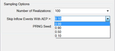
The skip inflow option, similar to number of realizations, should be chosen with consideration of simulation run time, accuracy, and project needs. If reservoir frequency relationships are only needed for extreme events, then it is recommended that a skip option of 0.10 is used. This will reduce run times while still producing accurate results for exceedance probabilities less than or equal to 0.10 (10-yr return period).
PRNG Seed
A seed is a number used to initialize the pseudorandom number generator (PRNG) in the stochastic simulation. The "auto" setting creates a default seed of 12345. The user can define a new PRNG seed if desired. The seed is used to initialize the PRNG sequence of random numbers. The same seed will always produce the exact same sequence of random numbers, thus producing the same simulation results (i.e., the seed ensures repeatability of results).
Output Options
- Frequency Curves
- Uncertainty bounds
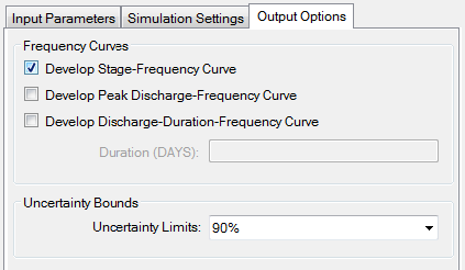
Frequency Curves
The user can select which frequency curves the simulation should develop. There are three options:
- Stage-Frequency Curve (this is the default)
- Peak Discharge-Frequency Curve
- Discharge-Duration-Frequency Curve
- This option requires a duration to be set. The RMC-RFA simulation framework relies on the critical duration. As such, discharge-duration-frequency curves will be more accurate for durations at least as long as the critical inflow duration.
Reservoir discharge-frequency relationships are often useful for assessing spillway erosion failure modes. For details on the plots created with each of these options see Frequency Curve Plots.
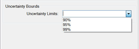
Uncertainty Bounds
RMC-RFA has three options availble for uncertainty limits during the simulation. The user should select one from the drop-down menu. 90% bounds are the default.
Tabular Results
Tabular Results displays the results for each realization and event simulated. The user can sort by any table header, by right clicking on the table header and selecting either Sort Ascending or Sort Descending.
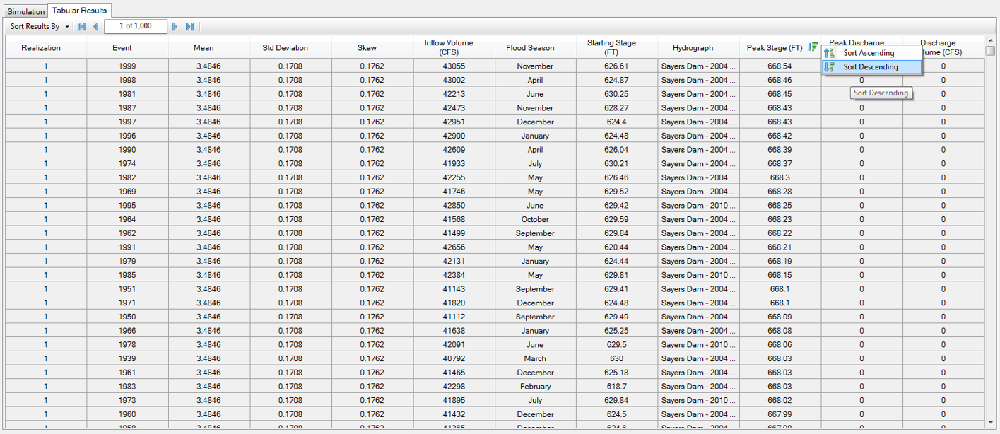
The user can also chose to Sort Results By: Realization or All Realizations. When the results are sorted by Realization, the arrows at the top of the window allow for scrolling through the different realizations.
Plot
- Frequency Curve Plots
- Simulated Input Plots
- Sensitivity Plots
- Routed Hydrograph Plots
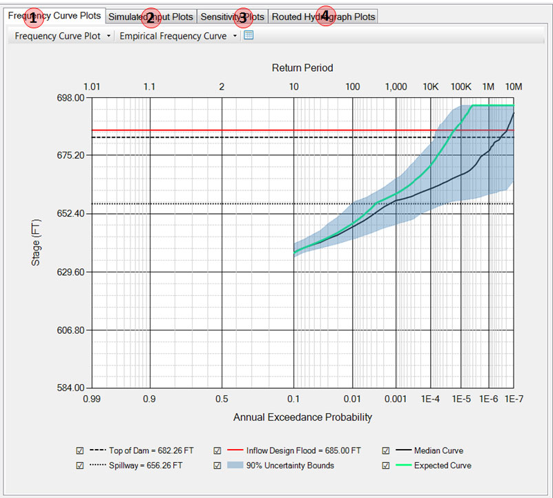
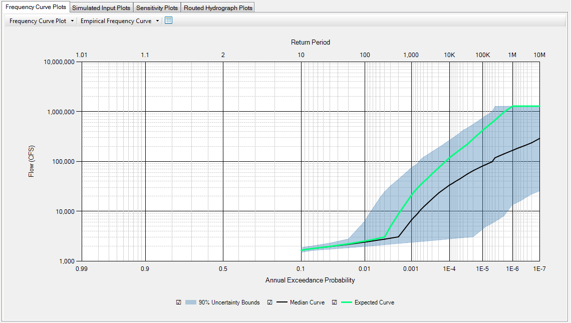
Frequency Curve Plots
Three Frequency Curve Plots are availabe:
- Stage-Frequency Curve
- Peak Discharge-Frequency Curve
- Discharge-Duration-Frequency Curve
The stage-frequency curve is the default curve developed following a simulation. In order to output the peak-discharge-frequency curve and the discharge-duration-frequency curve these need to be selected in Output Options.
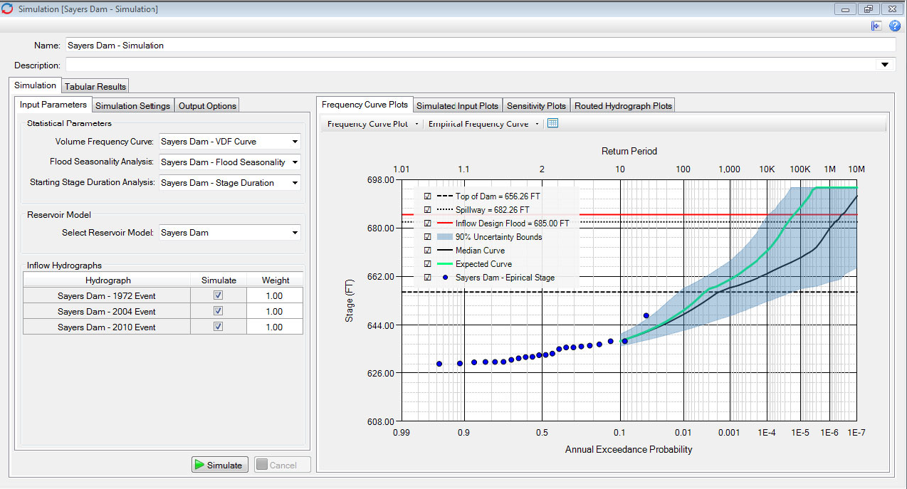
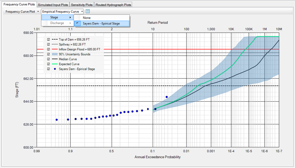
Additionally, Empirical Frequency Curves calculated in the Analyses can be displayed on the same plot as the frequency curve as shown below:
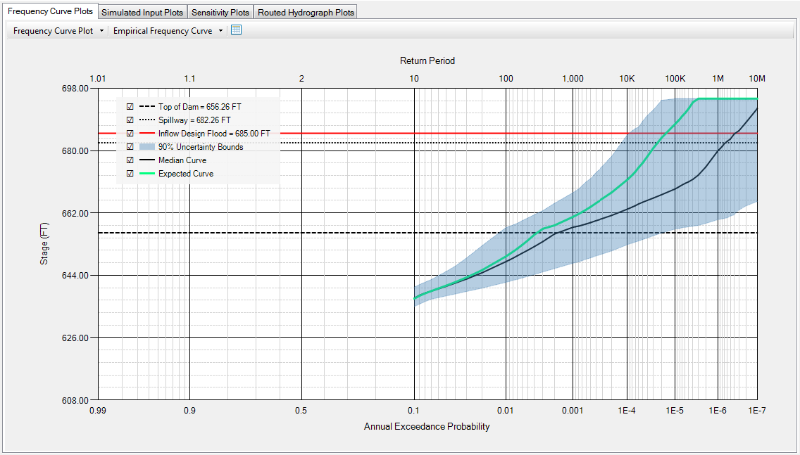
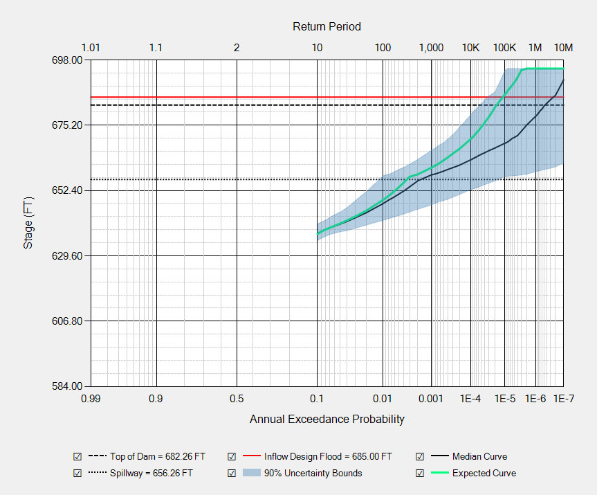
Stage-Frequency Curve
This plot is the default created with each simulation. Depending on the options selected, it shows the reservoir features, the median curve, the expected curve, and the uncertainty bounds. This plot has all of the same features discussed in Chart Features.
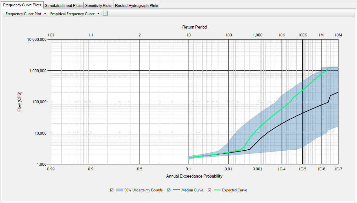
Peak Discharge-Frequency Curve
This is the peak discharge-frequency curve. It shows the median curve, expected curve, and uncertainty bounds. This plot has all of the same features discussed in Chart Features.
Discharge-Duration-Frequency Curve
This is the discharge-duration-frequency plot. It shows the median curve, expected curve, and uncertainty bounds for a specified duration. This plot has all of the same features discussed in Chart Features.
Results Empirical Frequency Curve
This option allows the user to display an empirical frequency curve along with the simulated curves. Stage is available for the Stage-Frequency plot, whereas Discharge is available for the Peak Discharge-Frequency plot and the Discharge-Duration-Frequency plot. This plot has all of the same features discussed in Chart Features.

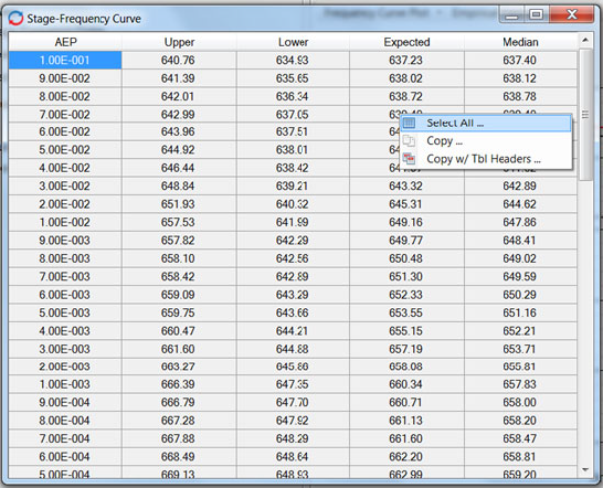
Tabular Output
Tabular output for each of the Frequency Curve Plots can be accessed with the tabular button. Whichever plot is displayed when the button is selected is tabulated. Once the tabular output window pops up, the user can right click within the window, and Select All, Copy and Copy with Table Headers.
Simulated Input Plots
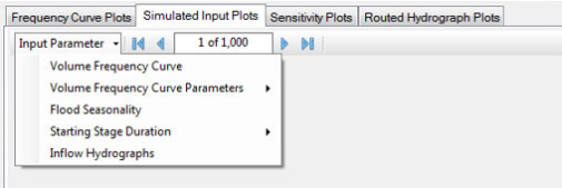
The following Simulated Input Plots are available:
- Volume Frequency Curve
- Volume Frequency Curve Parameters
- Mean
- Standard Deviation
- Skew
- Flood Seasonality
- Starting Stage Duration
- Inflow Hydrographs
The Simulated Input Plots compare the user defined parameters to the bootstrap sampled parameters used in the simulation for each realization. The user can scroll through the parameters for each realization using the arrows at the top of the window.
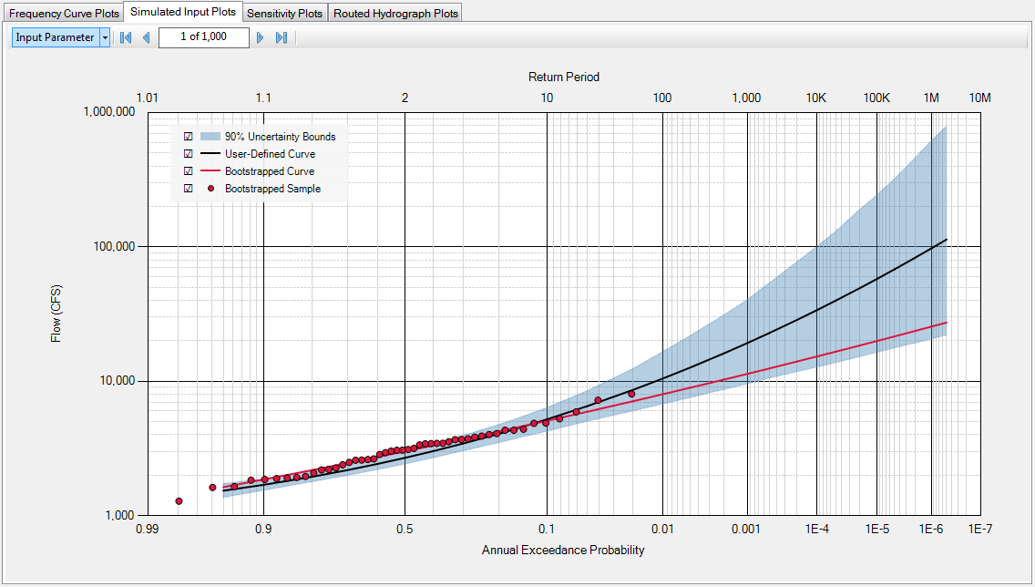
Volume Frequency Curve
The Volume-Frequency Curve plot displays the user-defined curve inflow volume-frequency curve compared to the bootstrapped curve and bootstrapped sample for a particular realization. It also shows the 90% confidence bounds. This plot has all of the same features discussed in Chart Features.
Volume Frequency Curve Parameters
Volume Frequency Curve Parameters has three variable options:
- Mean
- Standard Deviation
- Skew
This plot illustrates the knowledge uncertainty in the form of sampling error for the mean, standard deviation, and skew.
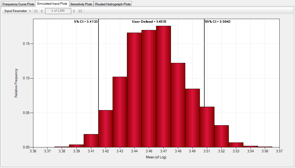
Mean
Volume Frequency Curve Parameters Mean plot displays the relative frequency of the mean (of log) compared to the user-defined mean and 90% confidence intervals. This plot has all of the same features discussed in Chart Features.
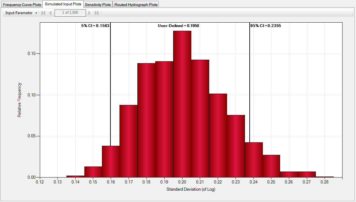
Standard Deviation
Standard Deviation plot displays the relative frequency of the standard deviation (of log) compared to the user-defined standard deviation and 90% confidence intervals. This plot has all of the same features discussed in Chart Features.
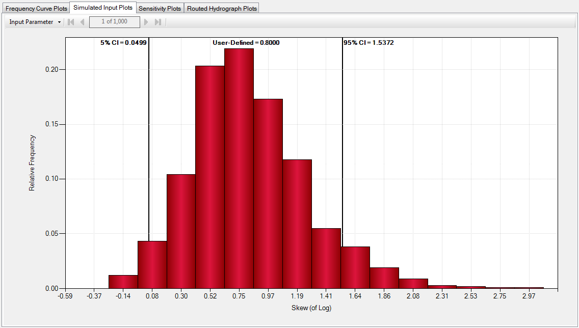
Skew
Skew plot displays the relative frequency of the skew (of log) compared to the user-defined skew and 90% confidence intervals. This plot has all of the same features discussed in Chart Features.
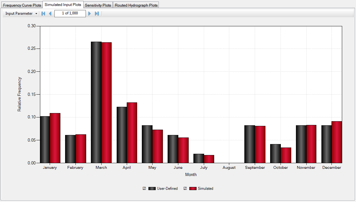
Flood Seasonality
The Flood Seasonality plot shows the relative frequency of events versus month for each realization. It displays the user-defined flood seasonality compared to the simulated seasonality. This plot has all of the same features discussed in Chart Features.
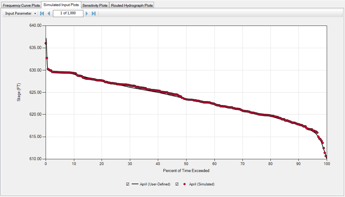
Starting Stage Duration
The Starting Stage Duration plot shows the stage versus the percent of time exceeded for each realization by month. It displays the user-defined starting stage duration to the simulated starting stage duration. This plot has all of the same features discussed in Chart Features.
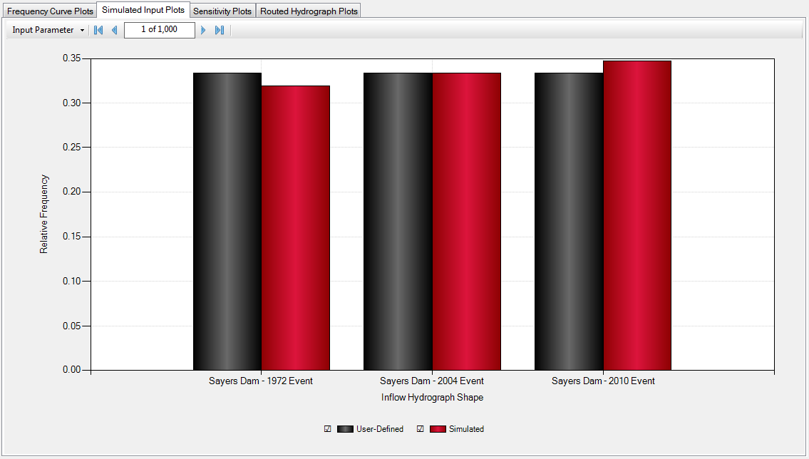
Inflow Hydrographs
The Inflow Hydrograph plot shows the relative frequency of each inflow hydrograph in the simulation by realization. It displays the user-defined inflow hydrograph frequency to the inflow hydrograph frequency. This plot has all of the same features discussed in Chart Features
Sensitivity Plots
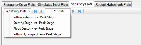
The following Sensitivity Plots are available:
- Inflow Volume -vs- Peak Stage
- Starting Stage -vs- Peak Stage
- Flood Season -vs- Peak Stage
- Inflow Hydrograph -vs- Peak Stage
The Sensitivity plots are calculated for each realization. The user can scroll through each realization using the arrows at the top of the window.
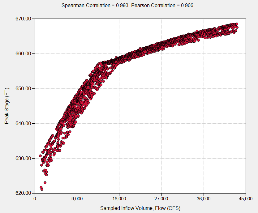
Inflow Volume -vs- Peak Stage
The Inflow Volume -vs- Peak Stage plot displays the sampled inflow volume versus the peak stage for each realization. It displays the Spearman Correlation and the Pearson Correlation. This plot has all of the same features discussed in Chart Features.
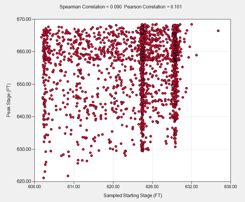
Starting Stage -vs- Peak Stage
The Starting Stage -vs- Peak Stage plot displays the sampled starting stage versus the peak stage for each realization. It displays the Spearman Correlation and the Pearson Correlation. This plot has all of the same features discussed in Chart Features.
Flood Season -vs- Peak Stage
The Flood Season -vs- Peak Stage plot displays the sampled month versus the peak stage for each realization in the form of a box and whisker plot. This plot has all of the same features discussed in Chart Features.
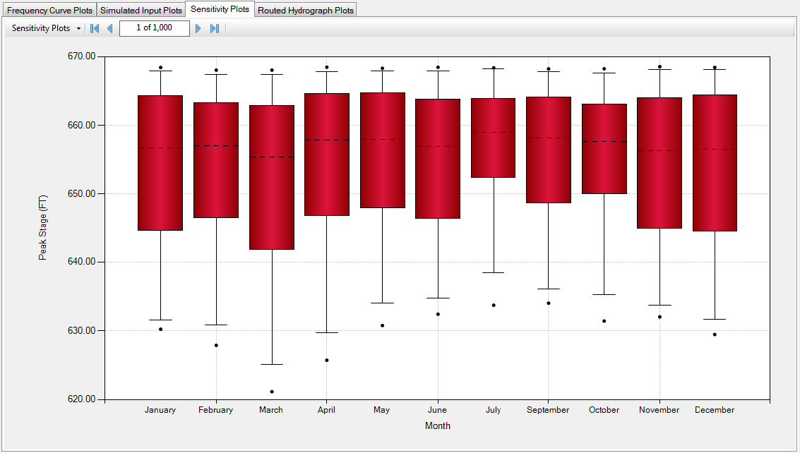
The box and whisker plot provides a seven number summary, where the two points represent the min and max, the whiskers represent the 5th and 95th percentiles, the box bottom and top represent the 25th and 75th percentiles respectively, and the dashed line represents the median.
Inflow Hydrograph -vs- Peak Stage
The Inflow Hydrograph -vs- Peak Stage plot displays the sampled inflow hydrograph versus the peak stage for each realization in the form of a box and whisker plot. This plot has all of the same features discussed in Chart Features.
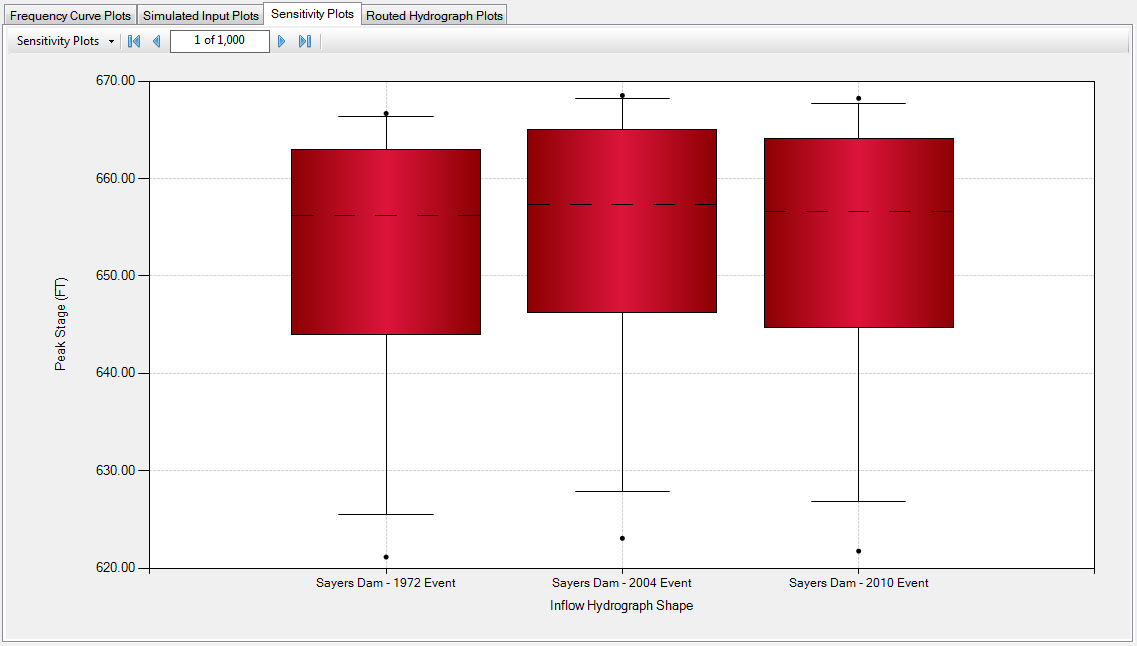
The box and whisker plot provides a seven number summary, where the two points represent the min and max, the whiskers represent the 5th and 95th percentiles, the box bottom and top represent the 25th and 75th percentiles respectively, and the dashed line represents the median.
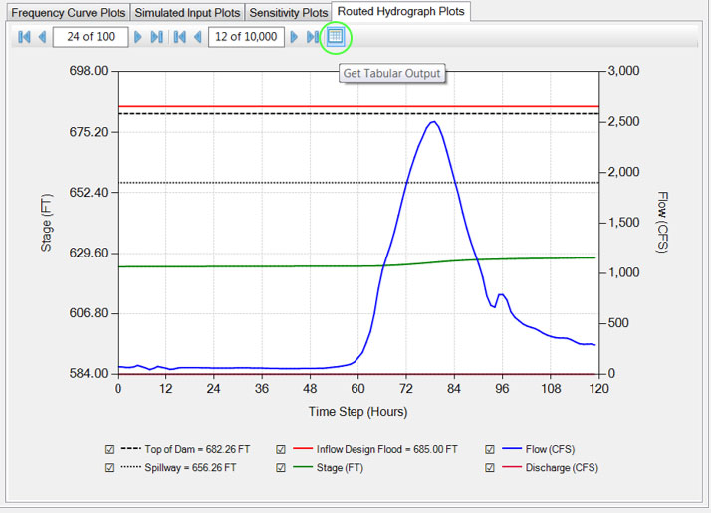
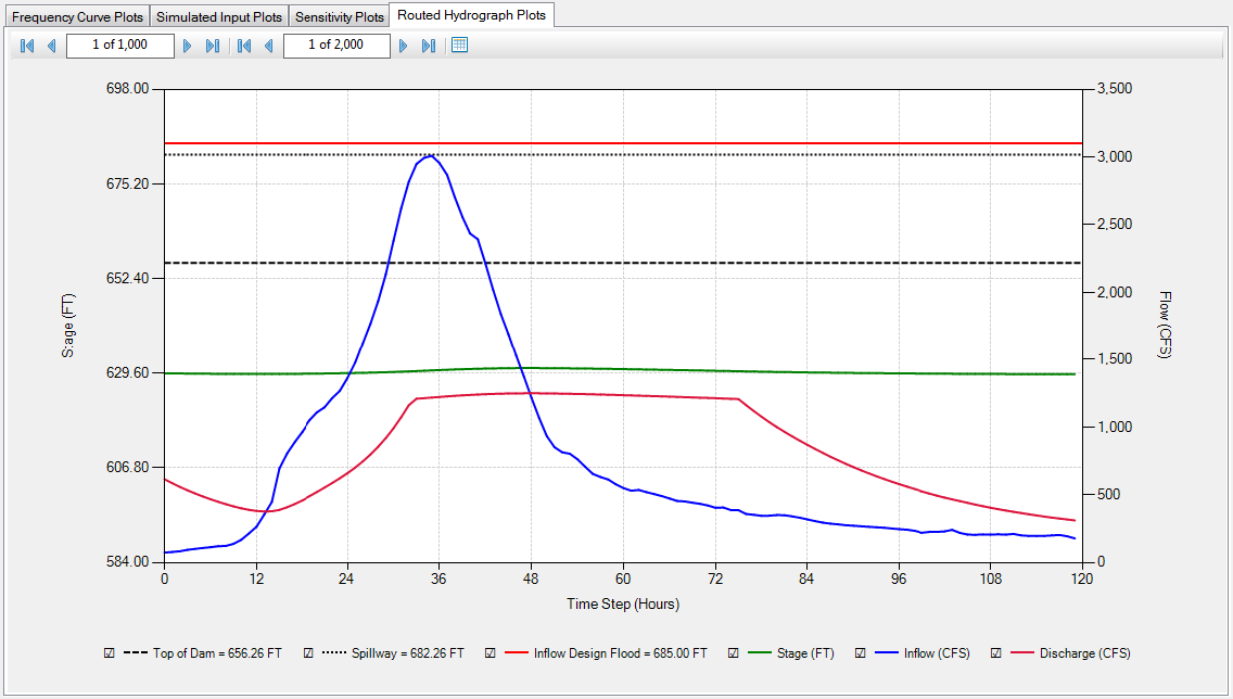
Routed Hydrograph Plots
Routed Hydrograph plots displays the inflow hydrograph routed through the reservoir model for each realization. It shows the inflow hydrograph, discharge, stage, and reservoir features. This plot has all of the same features discussed in Chart Features.
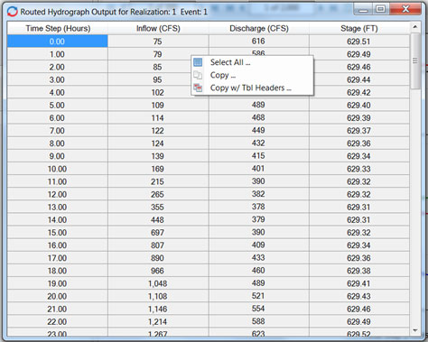
Tabular Output
Tabular output for each routed hydrograph plot can be accessed by hitting the tabular output button . Once the tabular output window opens, the user can select all, copy and copy with table headers by right clicking within the table.