Conceptual Computation of an rfaR Realization
Source:vignettes/rfaR-Realization-Conceptual.Rmd
rfaR-Realization-Conceptual.RmdExecutive Summary
RMC-RFA produces a reservoir stage-frequency curve with uncertainty bounds by utilizing a deterministic flood routing model within a nested Monte Carlo simulation. The nested Monte Carlo simulation quantifies natural variability and epistemic uncertainty by treating inflow volume, flood hydrograph shape, seasonal occurrence, and antecedent reservoir stage as uncertain variables.
The inner loop — defined here as a realization — simulates natural variability by routing 10,000 individual flood events through the reservoir, each with a randomly sampled starting stage, hydrograph shape, and inflow volume. Together the 10,000 routed events produce a single stage-frequency curve estimate. The outer loop propagates epistemic uncertainty by repeating this process across many realizations, each conditioned on a different set of volume-frequency distribution parameters drawn from the posterior.
This document walks through a single realization in detail.
Understanding one realization is the key to understanding the full
simulation: the outer loop repeats realizations with a resampled
parameter sets (in rfaR, this is the next
parameter set from the input). The walkthrough covers the stratified
sampling procedure, random sampling of starting stage and hydrograph
shape, and calculation of stage exceedance probabilities. These steps
are common to all simulation types. The full uncertainty simulation
conducts 10,000 realizations, each comprising 10,000 flood events (100
million routing operations total), while the expected value simulation
conducts 10,000 realizations, each using a one of the 10,000 BestFit
parameter sets.
Note: Users with coding experience may find the loops in this script “inefficient”. This purpose of this step-by-step guide is to provide a replicable guide to the realization process.
rfaR Analysis Summary
A full uncertainty run in rfa_simulate() is the result
of 10,000 realizations. An individual realization is comprised of 10,000
deterministic routing simulations. Each simulation contains:
Stratified sample from an inflow volume-frequency curve (VFC)1
Seasonality sample represented by the month
Starting stage sample, dependent on the sampled month
Hydrograph Shape, scaled to sampled inflow volume
Modified-Puls routing to obtain peak stages and/or peak discharge
These module emulate the workflow and methodology from RMC-RFA. The
subsections below will step through an rfaR realization. These sections
represent modules and functions contained in
rfa_simulate().
Flow-Frequency Stratified Sampling
Stratified Bins Definition & Set-Up
Stratified sampling is used instead of simple random sampling because
reliable estimates of exceedance probabilities far into the tail of the
distribution (events with AEPs of 1/10,000 or rarer) are required.
Simple random sampling would require an impractically large number of
events to adequately populate the tail. Instead, the frequency axis is
divided into equal-probability bins (Nbins), and events are
sampled uniformly within each bin (Mevents). This ensures
the tail is well-represented without artificially inflating the total
number of routing operations.
ords <- stratified_sampler(Nbins = 20, Mevents = 500, dist = "ev1")The bin weights (ords$Weights) reflect the true
probability mass that each bin represents. These weights are applied
later to reconstruct the true exceedance probability from the stratified
sample, correcting for the fact that rare-event bins were intentionally
oversampled relative to their actual frequency of occurrence.
Construct a Probability Matrix from the Stratified Bins
The z-variate matrix translates each stratified sample into a
standard normal deviate. Each column corresponds to one bin; each row is
one of the Mevents random draws within that bin. Because
EV1 (Gumbel) space is used for stratification, the bin boundaries
(Zlower, Zupper) are in defined in
Gumbel-reduced-variate space, and events are drawn uniformly within each
bin. The resulting z_matrix is an Mevents ×
Nbins matrix of z-variates, with each column densely and
uniformly populated across its corresponding probability/z-variate
range.
z_matrix <- matrix(ncol = ords$Nbins, nrow = ords$Mevents)

# Using EV1
for (i in 1:ords$Nbins) {
  # Lower Bin Boundary (prior bin's upper boundary)
  bin_lower <- ords$Zlower[i]

  # Upper Bin Boundary
  bin_upper <- ords$Zupper[i]

  # Vector of random values
  z_matrix[, i] <- (bin_lower +
    (runif(500, min = 0, max = 1)) * (bin_upper - bin_lower))
}
Construct a Matrix of Corresponding Flow Quantiles
The Z-variates are converted to inflow volumes using the LP3
(Log-Pearson Type III) quantile function. The conversion routes through
normal probability space: Z-variates → normal CDF (pnorm) →
LP3 quantile (qp3). The result is Q_matrix,
which has the same dimensions as z_matrix and each cell
holds an inflow volume. Each inflow volume corresponds to a sample from
the inflow volume-frequency distribution.
The parameter set used here (meanlog,
sdlog, skewlog) represents a single draw from
the distribution of LP3 parameters — one posterior parameter set for
this realization.
meanlog <- 3.550399
sdlog <- 0.3717982
skewlog <- 0.7555138

Q_matrix <- 10^qp3(pnorm(z_matrix), meanlog, sdlog, skewlog)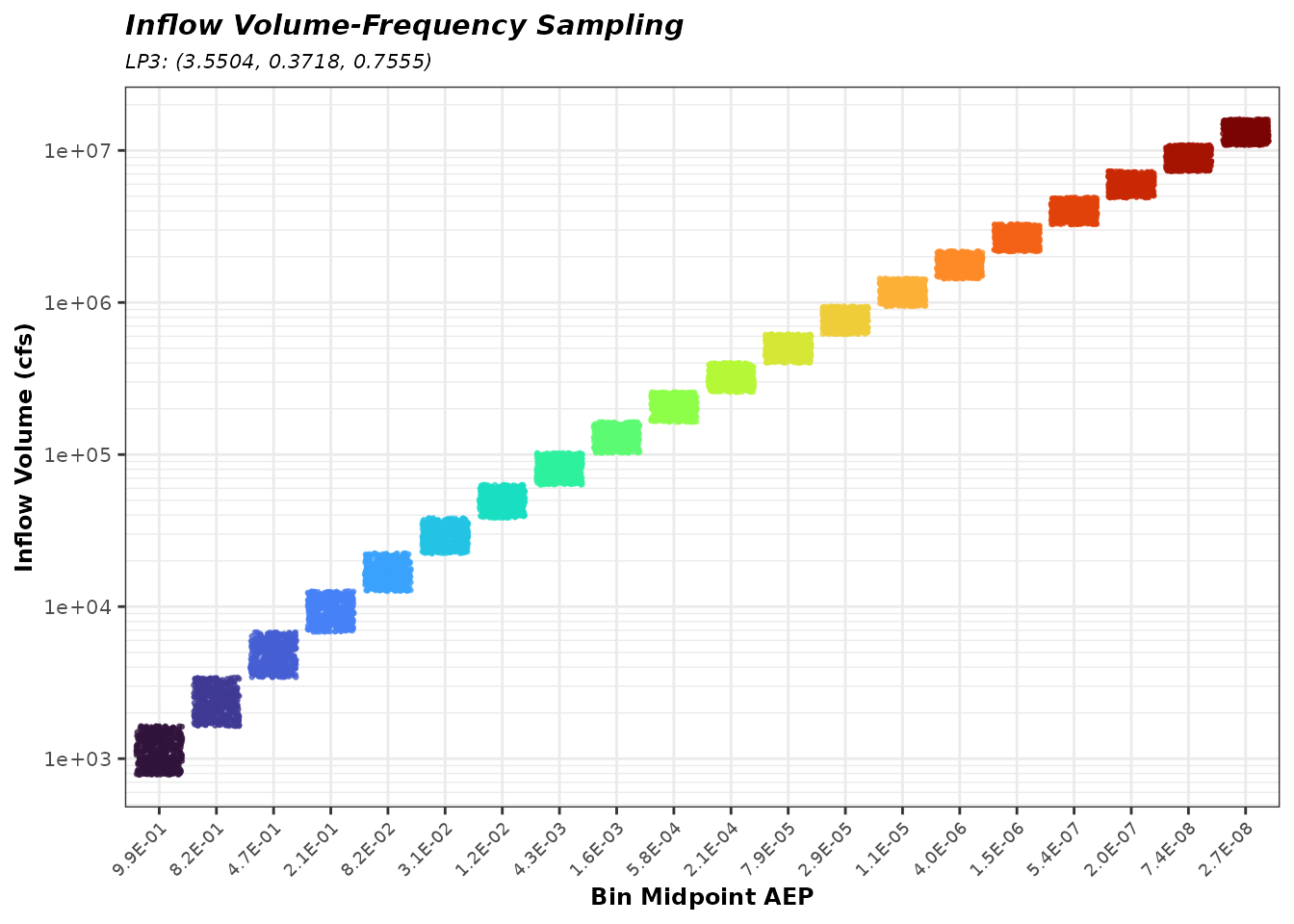
Define the Number of Simulations (Routings)
The total number of inflow events in this realization is the product of the number of bins and the number of events per bin — in this case, 20 × 500 = 10,000. This is the number of reservoir routing simulations that will be executed in the realization. The default is 10,00 simulations (equal to the number of parameter sets). Currently, there is no option to change the number of simulations or realizations.
Sample Seasonality
The month of flood occurrence is sampled randomly using historical relative frequencies from the site’s seasonal record. This captures the seasonal pattern of large inflow or high stage events. The sampled month is used in the next step to sample an observed starting reservoir stage that is climatologically consistent with the inflow timing, preserving the correlation between stage elevation and seasonality.
The sample is a pre-allocated vector/sequence of months that is
Nsims long.
InitMonths <- sample(
  1:12,
  size = Nsims,
  replace = TRUE,
  prob = jmd_seasonality$relative_frequency
)

UniqMonths <- sort(unique(InitMonths))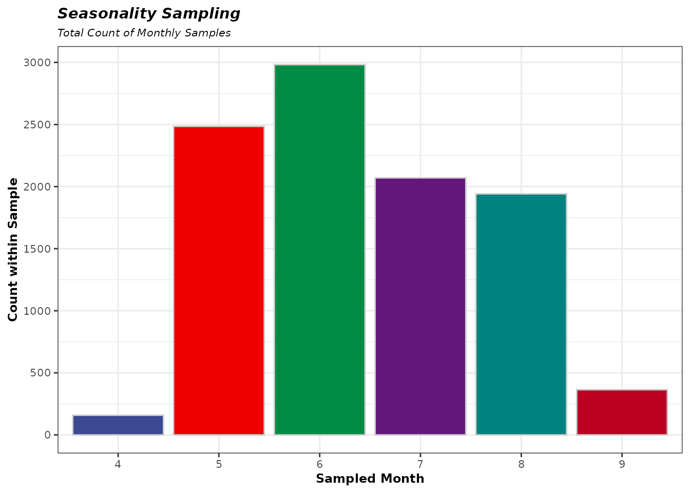
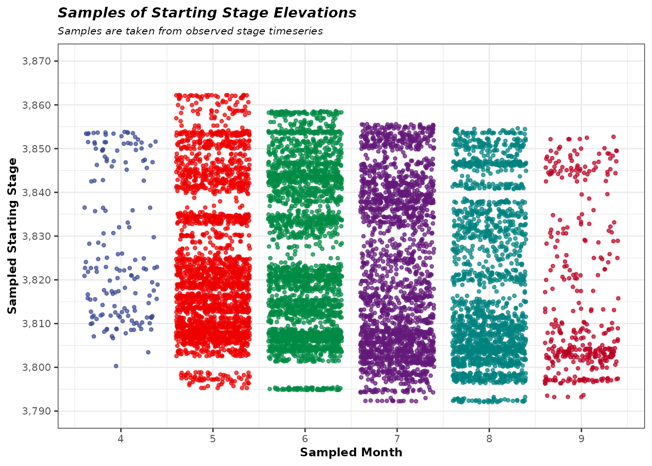
Sample Starting Stage
The antecedent reservoir stage for each event is sampled conditionally on the sampled month of occurrence. Observed stages are sampled from the month they occurred, using the sampled flood month in the step prior. This ensures that starting conditions are seasonally realistic — an event sampled in April will begin from a stage elevation sampled from April in the observed stage time series. The starting stages are therefore sampled proportionately to their historic frequency of occurrence.
The sample is a pre-allocated vector/sequence of starting stages that
is Nsims long.
InitStages <- numeric(Nsims)

stage_ts <- jmd_wy1980_stage
stage_ts$months <- lubridate::month(lubridate::mdy(stage_ts$date))

for (i in 1:length(UniqMonths)) {
  sampleID <- which(InitMonths == UniqMonths[i])
  InitStages[sampleID] <- sample(
    stage_ts$stage[stage_ts$months %in% UniqMonths[i]],
    size = sum(InitMonths == UniqMonths[i]),
    replace = TRUE
  )
}
Sample Hydrograph Shape
The shape of the flood hydrograph is sampled randomly from a
selection of historical and synthetic hydrographs. Each hydrograph in
the library is assigned a weight (default weights are uniform); the
sampled shape is then scaled to match the flood volume drawn from the
LP3 distribution. Note that the defined critical duration is 2-days
(critical_duration) and the routing window has been set to
10-days (routing_days).
hydrographs <- hydrograph_setup(
jmd_hydro_apr1999,
jmd_hydro_jun1921,
jmd_hydro_jun1965,
jmd_hydro_jun1965_15min,
jmd_hydro_may1955,
jmd_hydro_pmf,
jmd_hydro_sdf,
critical_duration = 2,
routing_days = 10
)
hydroSamps <- sample(
1:length(hydrographs),
size = Nsims,
replace = TRUE,
prob = attr(hydrographs, "probs")
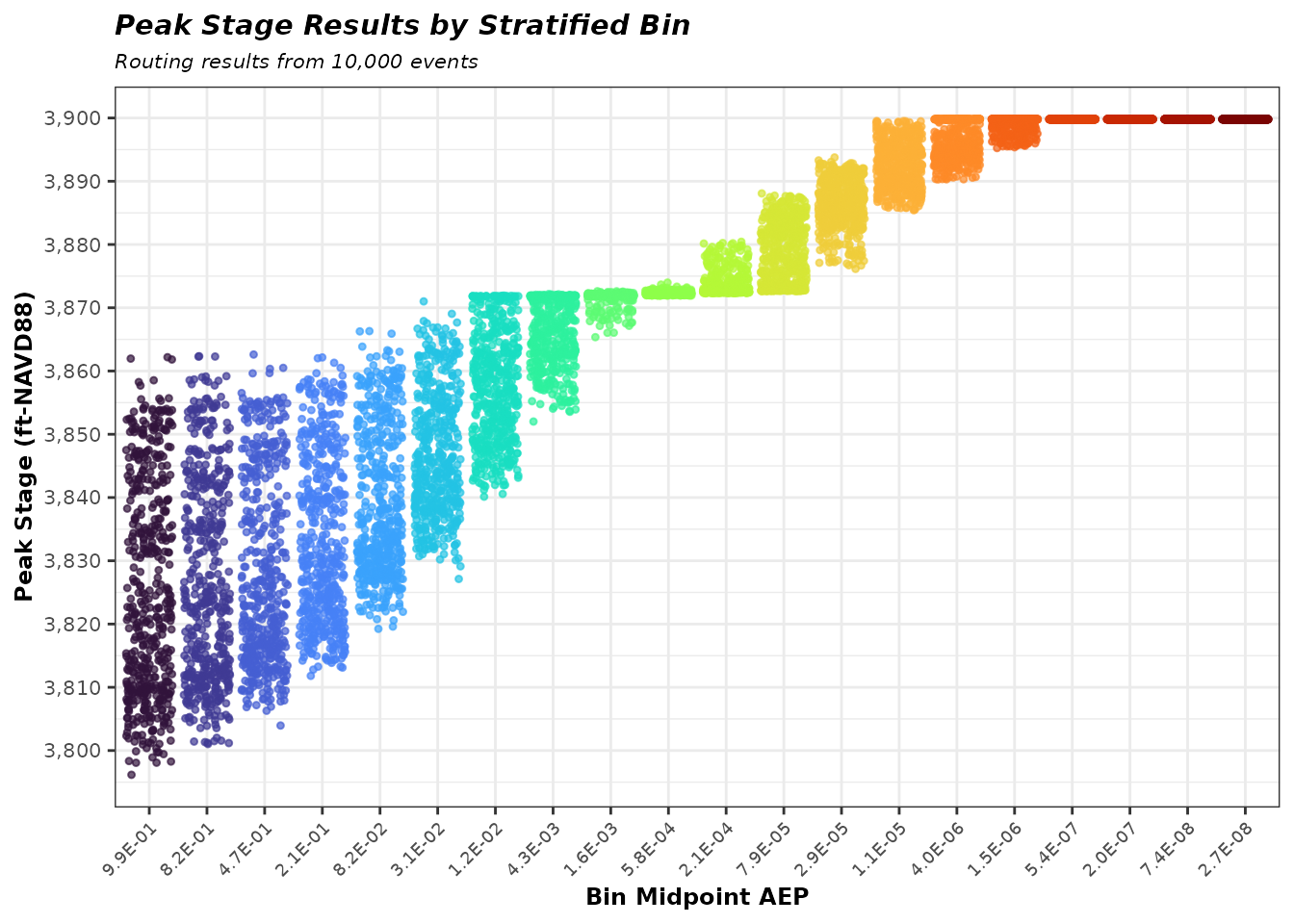
)Conduct Reservoir Routing Simulations
With all random variables sampled, the routing loop executes the
Modified Puls method for each of the Nsims events. For each
event, three inputs are combined: (1) the inflow hydrograph, scaled from
the sampled shape to match the LP3-derived inflow volume; (2) the
initial reservoir elevation drawn for that event; and (3) the
reservoir’s storage-outflow relationship (resmodel_df). The
Modified Puls method numerically solves the storage equation at each
timestep, tracking the reservoir elevation through the duration of the
flood. Only the peak stage reached during the event is retained in this
example, but peak discharge is also available.
The loop is structured to preserve the bin (column) alignment of
Q_matrix: event (i, j) in
peakStage corresponds to bin j and event
i. Maintaining this alignment is essential for correctly
applying the stratified bin weights during the stage-frequency
estimation.
peakStage <- matrix(NA, nrow = nrow(Q_matrix), ncol = ncol(Q_matrix))

realiz <- 0

for (i in 1:nrow(Q_matrix)) {
  for (j in 1:ncol(Q_matrix)) {
    # Keeps the indices lined up - necessary for the weights later
    realiz <- (i - 1) * ncol(Q_matrix) + j

    # Hydrograph shape
    hydrograph_shape <- hydrographs[[hydroSamps[realiz]]][, 2:3]

    # Hydrograph observed volume
    obs_hydrograph_vol <- attr(hydrographs[[hydroSamps[realiz]]], "obs_vol")

    # Scale hydrograph to sample volume
    scaled_hydrograph <- scale_hydrograph(
      hydrograph_shape,
      obs_hydrograph_vol,
      Q_matrix[i, j]
    )

    # Route scaled hydrograph
    tmpResults <- mod_puls_routing(
      resmodel_df = jmd_resmodel,
      inflow_df = scaled_hydrograph,
      initial_elev = InitStages[realiz],
      full_results = FALSE
    )

    # Record results
    peakStage[i, j] <- tmpResults[1]
  }
}
Realizaton Results
Determine Min and Max Stages
The range of routed peak stages defines the domain over which the realization stage-frequency curve will be estimated. All subsequent exceedance probability calculations (within the realization) are bounded by these values.
Define Exceedance Stages
A vector of stage thresholds is constructed by stepping evenly &
incrementally from the minimum to the maximum peak stage across the
number of events in each bin (Mevents). Each threshold in
stage_vect represents a candidate stage level at which
exceedance probability will be computed, forming the vertical axis of
the stage-frequency curve.
For consistency with code chunks, the candidate stages in
stage_vect can be referred to as “exceedance stages”. Note
that the vector of exceedance stages can be any length (ex.
n_exceedance_stages could be 1,000).
n_exceedance_stages <- ords$Mevents
stage_vect <- rep(NA, n_exceedance_stages)

for (b in 1:(n_exceedance_stages)) {
  # Min Stage
  if (b < 2) {
    stage <- min_stage

    # Incrementally calculate the next exceedance stage
  } else {
    stage <- stage_vect[b - 1] + (max_stage - min_stage) / (n_exceedance_stages)
  }
  stage_vect[b] <- stage
}
Count Exceedances & Relative Frequencies
For each bin (column) of peakStage and each exceedance
stage (exceedance_stage), the number of events with peak
stages greater than the exceedance stage is totaled and divided by the
number of events. This is the probability of exceeding a stage, given
that the inflow volume was drawn from that inflow volume-frequency bin.
The result is stored in stage_exceedance_matrix, with rows
corresponding to exceedance stages in stage_vect and
columns corresponding to stratified bins.
The accompanying graphic illustrates this process. In each bin, the
number of stages exceeding stage_vect[1] is summed by
stage_exceed_count. This is then divided by the number of
routed events in the bin (mstages) to represent a
probability of exceedance (stage_exceed_prob). This
processes is repeated for each exceedance stage in
stage_vect, within each bin.
stage_exceedance_matrix <- matrix(
  nrow = length(stage_vect),
  ncol = ncol(Q_matrix)
)

for (m in 1:ncol(peakStage)) {
  # Get Bin of peak stages, each represented by m event
  mstages <- peakStage[, m]

  for (n in 1:length(stage_vect)) {
    # Get Stage
    exceedance_stage <- stage_vect[n]

    # How many exceedances in Bin
    stage_exceed_count <- sum(mstages > exceedance_stage)

    # Exceedance Prob in Bin
    stage_exceed_prob <- stage_exceed_count / length(mstages)

    # Save to exceedance matrix
    stage_exceedance_matrix[n, m] <- stage_exceed_prob
  }
}
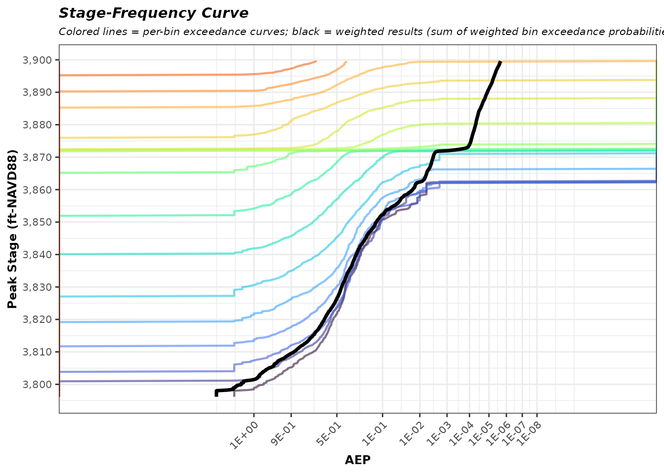
Estimate Exceedance Probabilities using Stratified Bin Weights
The stage exceedance probabilities from each bin are combined using the stratified bin weights. The weighted sum of bin-level exceedance probabilities estimates the annual exceedance probability (AEP) at a given exceedance stage. The weighted sum is to correct for the intentional oversampling of rare/less-frequent inflow events. For more on this see the Law of Total Probability.
The result is stage_result which is the stages from
stage_vect and their corresponding AEP estimates. This is
the realization stage-frequency curve. This curve can be interpolated
using stages or AEPs.
stage_aep_vect <- rep(NA, length(stage_vect))

for (m in 1:nrow(stage_exceedance_matrix)) {
  # Grab row of exceedances
  stage_exceedance_probs <- stage_exceedance_matrix[m, ]

  # Sum the dot product of exceedances and weights
  stage_aep <- sum(stage_exceedance_probs * ords$Weights)

  #save to vector
  stage_aep_vect[m] <- stage_aep
}

stage_result <- tibble(
  AEP = stage_aep_vect,
  Z_var = qnorm(1 - stage_aep_vect),
  Gumb = -log(-log(1 - AEP)),
  Stage = stage_vect
)
Concluding Remarks
Understanding the Role of a Single Realization
Understanding the inputs and calculation procedures of a single realization is crucial to understanding the nested Monte Carlo simulation process. Realization computations are used in both expected-only and full uncertainty stage-frequency estimates. The expected-only estimation consists of a single realization using 10,000 stratified volume-frequency samples, each drawn from an individual volume-frequency distribution parameter set. Full uncertainty computations perform one realization for each volume-frequency distribution parameter set to satisfy the law of total probability.
Deterministic Routing Within a Probabilistic Framework
RMC-RFA produces a reservoir stage-frequency curve with uncertainty bounds by employing a deterministic flood routing model within a nested Monte Carlo simulation. The inputs to each routing simulation are sampled probabilistically, while the reservoir model routes each simulated flood event using deterministic stage-storage-discharge functions.
The Law of Total Probability is the Theoretical Backbone
The nested Monte Carlo process provides reliable stage-frequency estimates with uncertainty bounds through the law of total probability. Complete integration over the sample space is achieved through stratified inflow-volume sampling within each volume-frequency parameter set, ensuring the full range of flood outcomes is represented across all parameter uncertainty.